Translucency and Subsurface Scattering
Translucency and Subsurface Scattering
October 2002 (Revised February 2013)
- 1 Introduction
- 2 Multiple scattering (diffusion approximation) with ptfilter
- 3 Multiple scattering with the subsurface() function
- 4 Smooth results even with sparse point clouds
- 5 Avoiding scattering across concavities
- 6 Ray-traced subsurface scattering
- 7 Single scattering
- 8 No scattering (absorption only)
- 9 Frequently Asked Questions
- 10 Improvements and extensions
1 Introduction
Subsurface scattering is an important effect for realistic rendering of translucent materials such as skin, flesh, fat, fruits, milk, marble, and many others. Subsurface scattering is responsible for effects like color bleeding inside materials, or the diffusion of light across shadow boundaries. The photograph below shows an example of translucent objects.
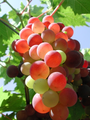
Translucent grapes
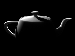
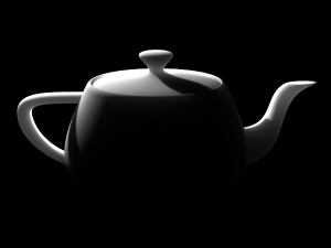
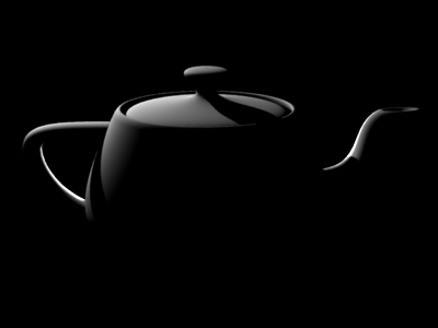
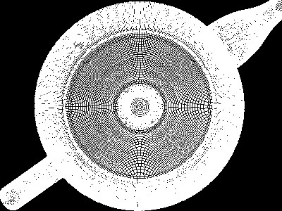
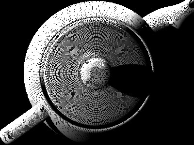
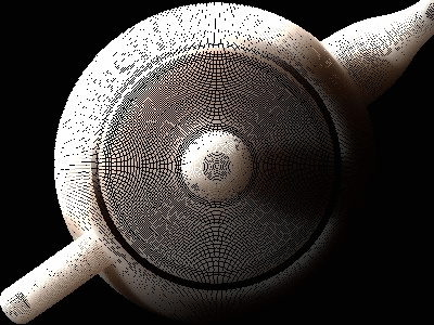
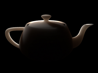
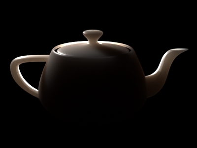
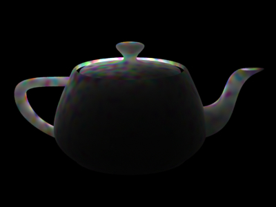
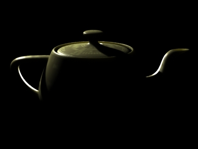
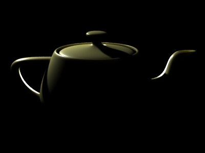
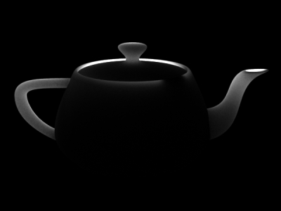
This application note describes how to simulate various aspects of subsurface scattering using Pixar's RenderMan (PRMan). The images below illustrate a simple example of subsurface scattering rendered with PRMan. The scene consists of a teapot made of a uniform, diffuse material. The teapot is illuminated by two spherical area lights (casting ray-traced shadows), one very bright light behind the teapot and another light to the upper left of the teapot. There is no subsurface scattering in the first image, so the parts of the teapot that are not directly illuminated are completely black. In the second image, the material of the teapot has subsurface scattering with a relatively short mean path length, so the light can penetrate thin parts, such as the handle, knob, and spout, but very little light makes it through the teapot body. In the third image, the mean path length is longer, so more light can penetrate the material and even the teapot body is brighter.

Direct illumination only |
With subsurface scattering (short mean path length) |
With subsurface scattering (long mean path length) |
In Section 2, we describe an efficient two-pass method to compute multiple scattering in a participating medium. In Section 7, we briefly discuss how to compute single scattering. In Section 8, we describe how to compute light transmission (without scattering) through a medium. Depending on the material parameters and the desired effects, one or several of these rendering methods can be chosen. For materials - such as human skin - that have high albedo, multiple scattering is much stronger than single scattering. In such cases, single scattering can be omitted.
2 Multiple scattering (diffusion approximation) with ptfilter
Multiple scattering is approximated as a diffusion process. This is done in four steps: 1) baking the diffuse surface transmission of direct illumination into a point cloud file; 2) diffusion simulation using the ptfilter program; 3) creating a brick map file; 4) rendering the final image with subsurface scattering.
2.1 Baking direct illumination
In the first step, the object is rendered with surface transmission of direct illumination, and one point per micropolygon is baked out to a point cloud file using the bake3d() shadeop. The shader looks like this:
surface
bake_radiance_t(string filename = "", displaychannels = ""; color Kdt = 1)
{
    color irrad, rad_t;
    normal Nn = normalize(N);
    float a = area(P, "dicing"); // micropolygon area

    /* Compute direct illumination (ambient and diffuse) */
    irrad = ambient() + diffuse(Nn);

    /* Compute the radiance diffusely transmitted through the surface.
       Kdt is the surface color (could use a texture for e.g. freckles).
       Alternatively, one can skip the multiplication by Kdt and just
       bake irradiance here.  (See discussion below.)
    */
    rad_t = Kdt * irrad;

    /* Store in point cloud file */
    bake3d(filename, displaychannels, P, Nn, "interpolate", 1,
           "_area", a, "_radiance_t", rad_t);

    Ci = rad_t * Cs * Os;
    Oi = Os;
}
We bake out the area at each point. The area is needed for the subsurface scattering simulation. NOTE: It is important for the area() function to have "dicing" as its optional second parameter. This ensures that the shader gets the actual micropolygon areas instead of a smoothed version that is usually used for shading. (Alternatively, the shader can be compiled with the -nosd option to get the same (non-smoothed) micropolygon areas from the area() function.) Without this, the areas will be, in general, too large, resulting in subsurface scattering simulation results that are too bright.
The optional parameter "interpolate" makes bake3d() write out a point for each micropolygon center instead of one point for each shading point. This ensures that there are no duplicate points along shading grid edges.
To ensure that all shading points are shaded, we set the attributes "cull" "hidden" and "cull" "backfacing" to 0 in the RIB file. We also set the attribute "dice" "rasterorient" to 0 to ensure an even distribution of shading points over the surface of the object. The RIB file for baking the diffusely transmitted direct illumination on a teapot looks like this:
FrameBegin 1

  Format 400 300 1
  シェーディングInterpolation "smooth"
  PixelSamples 4 4
  Display "teapot_bake_rad_t.rib" "it" "rgba"   # render image to 'it'
  Projection "perspective" "fov" 18
  Translate 0 0 170
  Rotate -15  1 0 0
  DisplayChannel "float _area"
  DisplayChannel "color _radiance_t"

  WorldBegin

    Attribute "visibility" "transmission" 1
    Attribute "trace" "bias" 0.01
    Attribute "cull" "hidden" 0   # don't cull hidden surfaces
    Attribute "cull" "backfacing" 0   # don't cull backfacing surfaces
    Attribute "dice" "rasterorient" 0   # turn view-dependent dicing off

    # Light sources (with ray traced shadows)
    LightSource "pointlight_rts" 1 "from" [-60 60 60] "intensity" 10000 "samples" 4
    LightSource "pointlight_rts" 2 "from" [0 0 100] "intensity" 75000 "samples" 4

    # Teapot
    AttributeBegin
      Surface "bake_radiance_t" "filename" "direct_rad_t.ptc"
                                "displaychannels" "_area,_radiance_t"
      Translate -2 -14 0
      Rotate -90  1 0 0
      Scale 10 10 10   # convert units from cm to mm
      Sides 1
      ジオメトリ "teapot"
    AttributeEnd

  WorldEnd
FrameEnd
The rendered image looks like this:
Diffuse surface reflection of direct illumination on teapot
This image is rather irrelevant; what we really care about is the generated point cloud file, direct_rad_t.ptc. The point cloud file has approximately 170,000 points with _radiance_t color values. Displaying the file with ptviewer and rotating it a bit gives the following view:
Point positions |
Points with _radiance_t values |
The point density is determined by the image resolution and the shading rate. If the points are too far apart, the final image will have low frequency artifacts. As a rule of thumb, the shading points should be spaced no more apart than the mean free path length lu (see the following).
In this example, the illumination is direct illumination from two point lights. It could just as well be high dynamic range illumination from an environment map or global illumination taking indirect illumination of the teapot into account.
2.2 Diffusion simulation using ptfilter
The volume diffusion computation is done using a stand-alone program called ptfilter. The diffusion approximation follows the method described in [Jensen01], [Jensen02], and [Hery03], and uses the same efficient algorithm as was used for, e.g., Dobby in Harry Potter and the Chamber of Secrets and Davy Jones and his crew in Pirates of the Caribbean: Dead Man's Chest.
The subsurface scattering properties of the material can be specified in three equivalent ways:
The simplest is to just specify a material name:
ptfilter -filter ssdiffusion -material marble direct_rad_t.ptc ssdiffusion.ptc
The built-in materials are apple, chicken1, chicken2, ketchup, marble, potato, skimmilk, wholemilk, cream, skin1, skin2, and spectralon; the data values are from [Jensen01]. The data values assume that the scene units are mm; if this is not the case, a unitlength parameter can be passed to ptfilter. For example, if the scene units are cm, use -unitlength 0.1.
Specify the reduced scattering coefficients (sigma's), absorption coefficients (sigmaa), and index of refraction of the material:
ptfilter -filter ssdiffusion -scattering 2.19 2.62 3.00 -absorption 0.0021 0.0041 0.0071 -ior 1.5 direct_rad_t.ptc ssdiffusion.ptc
Specify the diffuse color (BRDF albedo), diffuse mean free path lengths (in mm), and index of refraction of the material:
ptfilter -filter ssdiffusion -albedo 0.830 0.791 0.753 -diffusemeanfreepath 8.51 5.57 3.95 -ior 1.5 direct_rad_t.ptc ssdiffusion.ptc
The default material is marble.
The resulting point cloud file, ssdiffusion.ptc, has a subsurface scattering color ("_ssdiffusion") at every point:
Subsurface scattering diffusion values
The accuracy of the subsurface diffusion simulation can be determined by the ptfilter parameter "-maxsolidangle". This parameter determines which groups of points can be clustered together for efficiency. (It corresponds to the 'eps' parameter of [Jensen02], page 579.) This parameter is a time/quality knob: the smaller the value of maxsolidangle, the more precise (but slow) the simulation is. Values that are too large result in low-frequency banding artifacts in the computed scattering values. The default value for maxsolidangle is 1.
Tip
If you'd like to know which values of albedo, diffuse mean free path length, and index of refraction are being used for the subsurface diffusion simulation, you can add '-progress 1' to the ptfilter command line arguments. In addition, '-progress 2' will write out some of the computed subsurface scattering values.
On a multithreaded computer, the ptfilter computation can be sped up by giving the command line parameter "-threads *n*". The default is 1 thread.
2.3 Creating a brick map
Next, the point cloud file with subsurface diffusion colors needs to be converted to a brick map file so that the texture3d() shadeop can read it efficiently. This is done as follows:
brickmake -maxerror 0.002 ssdiffusion.ptc ssdiffusion.bkm
The top 3 levels of the resulting brick map, ssdiffusion.bkm, are shown below (visualized with the interactive brickviewer program):
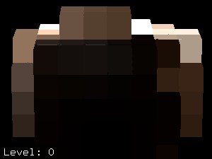
Brick map level 0 |
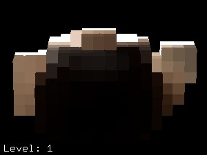
Brick map level 1 |
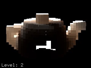
Brick map level 2 |
At level 2 you can see some of the bright voxels on the back side of the teapot body. This is because there are no brick voxels at that level in front of it (since those parts of the teapot body are uniformly dark.)
2.4 レンダリング subsurface scattering
We are finally ready to render the image with the subsurface scattering. The subsurface colors are read using the texture3d() function as in the following shader:
surface
read_ssdiffusion(uniform string filename = "";
                 float Ka = 1, Kd = 0, Ks = 1, roughness = 0.1)
{
    normal Nn = normalize(N);
    vector V = -normalize(I);
    color amb, diff, spec, ssdiffusion = 0;

    /* Compute direct illumination (ambient, diffuse, and specular) */
    amb = Ka * ambient();
    diff = Kd * diffuse(Nn);
    spec = Ks * specular(Nn, V, roughness);

    /* Look up subsurface scattering color */
    texture3d(filename, P, N, "_ssdiffusion", ssdiffusion);

    /* Set Ci and Oi */
    Ci = (amb + diff + ssdiffusion) * Cs + spec;
    Ci *= Os;
    Oi = Os;
}
The RIB file looks like this (the light sources are only needed for the direct illumination):
FrameBegin 1

  Format 600 450 1
  シェーディングInterpolation "smooth"
  PixelSamples 4 4
  Display "teapot_read_ssdiffusion.rib" "it" "rgba"   # render image to 'it'
  Projection "perspective" "fov" 18
  Translate 0 0 170
  Rotate -15  1 0 0

  WorldBegin

    Attribute "visibility" "transmission" 1
    Attribute "trace" "bias" 0.01

    # Light sources (with ray traced shadows)
    LightSource "pointlight_rts" 1 "from" [-60 60 60] "intensity" 10000 "samples" 4
    LightSource "pointlight_rts" 2 "from" [0 0 100] "intensity" 75000 "samples" 4

    # Teapot
    AttributeBegin
      Surface "read_ssdiffusion" "filename" "ssdiffusion.bkm"
      Translate -2 -14 0
      Rotate -90  1 0 0
      Scale 10 10 10   # convert units from cm to mm
      Sides 1
      ジオメトリ "teapot"
    AttributeEnd

  WorldEnd
FrameEnd
The subsurface scattering image looks like this (with and without specular highlights):
Subsurface scattering |
Subsurface scattering and specular highlights |
If desired, the shader can of course multiply the subsurface color by a texture, etc.
2.5 Varying albedo and diffuse mean free path length
The example above had a uniform albedo and a uniform diffuse mean free path length. It is simple to multiply the transmitted radiance by a varying diffuse color prior to baking it. For another effect, we can also specify varying albedos and diffuse mean free paths in the diffusion simulation. This requires that we bake the albedo and diffuse mean free paths in the point cloud file along with the transmitted radiance.
Shader example:
surface
bake_sss_params(string filename = "", displaychannels = ""; color Kdt = 1)
{
    color irrad, rad_t;
    color albedo, dmfp = 10;
    normal Nn = normalize(N);
    point Pobj = transform("object", P);
    float a = area(P, "dicing"); // micropolygon area
    float freq = 5;

    /* Compute direct illumination (ambient and diffuse) */
    irrad = ambient() + diffuse(Nn);

    /* Compute the radiance diffusely transmitted through the surface.
       Kdt is the surface color (could use a texture for e.g. freckles) */
    rad_t = Kdt * irrad;

    albedo = noise(freq * Pobj);

    /* Store in point cloud file */
    bake3d(filename, displaychannels, P, Nn, "interpolate", 1,
           "_area", a, "_radiance_t", rad_t, "_albedo", albedo,
           "_diffusemeanfreepath", dmfp);

    Ci = rad_t * Cs * Os;
    Oi = Os;
}
The RIB file is very much as in the previous example, but with more DisplayChannels and the bake_sss_params surface shader:
FrameBegin 1

  Format 400 300 1
  シェーディングInterpolation "smooth"
  PixelSamples 4 4
  Display "teapot_bake_rad_t.rib" "it" "rgba"   # render image to 'it'
  Projection "perspective" "fov" 18
  Translate 0 0 170
  Rotate -15  1 0 0
  DisplayChannel "float _area"
  DisplayChannel "color _radiance_t"
  DisplayChannel "color _albedo"
  DisplayChannel "color _diffusemeanfreepath"

  WorldBegin

    Attribute "visibility" "int diffuse" 1   # make objects visible for raytracing
    Attribute "visibility" "int specular" 1
    Attribute "visibility" "int transmission" 1
    Attribute "shade" "string transmissionhitmode" "primitive"
    Attribute "trace" "bias" 0.01
    Attribute "cull" "hidden" 0   # don't cull hidden surfaces
    Attribute "cull" "backfacing" 0   # don't cull backfacing surfaces
    Attribute "dice" "rasterorient" 0   # turn view-dependent dicing off

    # Light sources (with ray traced shadows)
    LightSource "pointlight_rts" 1 "from" [-60 60 60] "intensity" 10000 "samples" 4
    LightSource "pointlight_rts" 2 "from" [0 0 100] "intensity" 75000 "samples" 4

    # Teapot
    AttributeBegin
      Surface "bake_sss_params" "filename" "direct_and_params.ptc"
          "displaychannels" "_area,_radiance_t,_albedo,_diffusemeanfreepath"
      Translate -2 -14 0
      Rotate -90  1 0 0
      Scale 10 10 10   # convert units from cm to mm
      Sides 1
      ジオメトリ "teapot"
    AttributeEnd

  WorldEnd
FrameEnd
レンダリング this RIB file produces the point cloud file direct_and_params.ptc.
The diffusion simulation is done by calling ptfilter like this:
ptfilter -filter ssdiffusion -albedo fromfile -diffusemeanfreepath fromfile direct_and_params.ptc ssdiffusion.ptc
The resulting point cloud file, ssdiffusion.ptc, has a varying ssdiffusion color. The point cloud is converted to a brick map just as before:
brickmake -maxerror 0.002 ssdiffusion.ptc ssdiffusion.bkm
レンダリング the brick map is done using the same RIB file as in Section 2.4. The resulting image (without direct illumination) looks like this:
Subsurface scattering with varying albedo
Here are a couple of other images of subsurface scattering with varying albedo:
Direct illumination and subsurface scattering with varying albedo
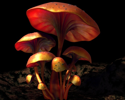
Mushrooms with direct illumination and subsurface scattering
-scattering and -absorption can also be read from a file using the fromfile syntax. These data must be baked into point cloud channels called "_scattering" and "_absorption".
2.6 Where to apply the surface albedo
It is easy be get confused about where to multiply by the surface albedo: where the light enters the surface, where it leaves the surface (the shading point), or both.
There are three choices:
- Multiply the incident illumination by the surface albedo when baking the point cloud. Use albedo 0.999 at the shading point.
- Multiply the incident illumination by the square root of the surface albedo when baking. Use the square root of the albedo at the shading point.
- Bake pure incident illumination into the point cloud -- do not multiply by albedo. Use the albedo at the shading point.
All three choices have some advantages and can be defended. It basically boils down to whether you want to emphasize the texture at the incident points or at the shading point. It would be wrong to use the full albedo at both places -- that results in an over-saturated subsurface color.
Choice 3) allows the highest frequency content in the subsurface results: if your skin albedo texture has a freckle you get a clear crisp freckle in the sss result, not a blurred-out soft spot. With 1) the textures' influence on the subsurface results get very blurry.
We chose the name "diffusely transmitted radiance" ("_radiance_t") thinking mainly of approach number 1). In hindsight, we could have chosen the name "_irradiance" for approach number 3) to make it clear that no albedo should be incorporated into it; that would also be more consistent with the ray-traced subsurface shader workflow.
2.7 Blocking geometry (internal structure)
The diffusion approximation described above can not take blocking geometry such as bones into account. But sometimes we would like to fake the effect of less subsurface scattering in e.g. skin regions near a bone. This can be done by baking negative illumination values on the internal object; this negative subsurface scattering will make the desired regions darker.
The same shader as above, bake_radiance_t, is used to bake the illuminated surface colors. But in addition, we use a simple shader to bake constant (negative, in this case) colors on the blocker:
surface
bake_constant( uniform string filename = "", displaychannels = "" )
{
    color surfcolor = Cs;
    normal Nn = normalize(N);
    float a = area(P, "dicing"); // micropolygon area

    bake3d(filename, displaychannels, P, Nn, "interpolate", 1,
           "_area", a, "_radiance_t", surfcolor);

    Ci = Cs * Os;
    Oi = Os;
}
Here is a RIB file for baking direct illumination on a thin box and negative color on a torus inside the box:
FrameBegin 1

   Format 300 300 1
   シェーディングInterpolation "smooth"
   PixelSamples 4 4
   Display "blocker_bake.rib" "it" "rgba"
   Projection "perspective" "fov" 15
   Translate 0 0 100
   Rotate -15  1 0 0

   DisplayChannel "float _area"
   DisplayChannel "color _radiance_t"

   WorldBegin

     Attribute "cull" "hidden" 0   # don't cull hidden surfaces
     Attribute "cull" "backfacing" 0   # don't cull backfacing surfaces
     Attribute "dice" "rasterorient" 0   # turn view-dependent dicing off

     # Light sources
     LightSource "pointlight" 1 "from" [-60 60 60] "intensity" 10000
     LightSource "pointlight" 2 "from" [0 0 100] "intensity" 75000

     # Thin box (with normals pointing out)
     AttributeBegin
       Surface "bake_radiance_t" "filename" "blocker_direct.ptc"
                                 "displaychannels" "_area,_radiance_t"
       Scale 10 10 2
       Polygon "P" [ -1 -1 -1  -1 -1 1  -1 1 1  -1 1 -1 ]   # left side
       Polygon "P" [ 1 1 -1  1 1 1  1 -1 1  1 -1 -1 ]       # right side
       Polygon "P" [ -1 1 -1  1 1 -1  1 -1 -1  -1 -1 -1 ]   # front side
       Polygon "P" [ -1 -1 1  1 -1 1  1 1 1  -1 1 1 ]       # back side
       Polygon "P" [ -1 -1 -1  1 -1 -1  1 -1 1  -1 -1 1 ]   # bottom
       Polygon "P" [ -1 1 1  1 1 1  1 1 -1  -1 1 -1 ]       # top
     AttributeEnd

     # Blocker: a torus with negative color
     AttributeBegin
       Surface "bake_constant" "filename" "blocker_direct.ptc"
                               "displaychannels" "_area,_radiance_t"
       カラー [-2 -2 -2]
       #カラー [-5 -5 -5]
       Torus 5.0 0.5  0 360  360
     AttributeEnd

   WorldEnd
 FrameEnd
レンダリング this RIB file results in a rather uninteresting image and a more interesting point cloud file called blocker_direct.ptc.
The next step is to do the subsurface scattering simulation. For this example we'll use the default material parameters. In order to avoid blocky artifacts it is necessary to specify a rather low maxsolidangle:
ptfilter -filter ssdiffusion -maxsolidangle 0.3 blocker_direct.ptc blocker_sss.ptc
Then a brick map is created from the subsurface scattering point cloud:
brickmake blocker_sss.ptc blocker_sss.bkm
To render the box with subsurface scattering we use the same shader, read_ssdiffusion, as in the previous sections. The RIB file looks like this:
FrameBegin 1

  Format 300 300 1
  シェーディングInterpolation "smooth"
  PixelSamples 4 4
  Display "blocker_read.rib" "it" "rgba"
  Projection "perspective" "fov" 15
  Translate 0 0 100
  Rotate -15  1 0 0

  WorldBegin

    Surface "read_ssdiffusion" "filename" "blocker_sss.bkm"

    # Thin box (with normals pointing out)
    AttributeBegin
      Scale 10 10 2
      Polygon "P" [ -1 -1 -1  -1 -1 1  -1 1 1  -1 1 -1 ]   # left side
      Polygon "P" [ 1 1 -1  1 1 1  1 -1 1  1 -1 -1 ]       # right side
      Polygon "P" [ -1 1 -1  1 1 -1  1 -1 -1  -1 -1 -1 ]   # front side
      Polygon "P" [ -1 -1 1  1 -1 1  1 1 1  -1 1 1 ]       # back side
      Polygon "P" [ -1 -1 -1  1 -1 -1  1 -1 1  -1 -1 1 ]   # bottom
      Polygon "P" [ -1 1 1  1 1 1  1 1 -1  -1 1 -1 ]       # top
    AttributeEnd

  WorldEnd
FrameEnd
Here are three images of the thin box with varying degrees of blocking:
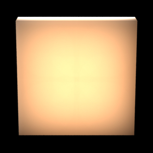
No blocking |
Blocking by torus with color [-2 -2 -2] |
Blocking by torus with color [-5 -5 -5] |
See [Hery03] for more discussion and examples of blocking geometry.
3 Multiple scattering with the subsurface() function
Multiple scattering can be computed more conveniently with the subsurface() function. The baking step is the same as described above. The ptfilter step is faster since ptfilter is only used to organize the point cloud - it does not compute any subsurface scattering at the points. (If the point cloud is small, the ptfilter step can even be omitted entirely.) The brick map step is skipped, and the subsurface scattering is computed during rendering with the subsurface() function. In the following, we will go through each step in more detail.
3.1 ptfilter partial computation
In order to enable the subsurface() function to read only parts of the point cloud file at a time, the point cloud needs to be preprocessed using ptfilter. (The preprocessing consists of organizing the points into an octree and computing the total area and power of the points in each octree node.) We tell ptfilter that we only need it to do a partial evaluation of the subsurface scattering (rather than a full computation at every point) by setting the command line parameter -partial to 1. The precomputation is independent of the material scattering parameters, so it is not necessary to specify them. Here is an example of such a call to ptfilter:
ptfilter -filter ssdiffusion -partial 1 direct_rad_t.ptc ssdiffusion.optc
(We often use a .optc suffix for organized point clouds.) The contents of the generated file, ssdiffusion.optc, can be inspected with ptviewer -info. It contains points with _area and _radiance_t data and octree nodes with bounding box, centroid, sumarea, and sumpower data.
Please note that this step is optional. If point cloud memory use is not an issue (the point cloud contains only a few million points) or if the rendering is only done a few times, it may not be worthwhile.
3.2 The subsurface() function
The input to the subsurface function is the position and normal, and the name of the point cloud file. The point cloud file must contain float area and color radiance data: the area and transmitted direct illumination at each point. (The default names are "_area" and "_radiance_t"; different channel names can be specified with the "areachannel" and "radiancechannel" parameters.) Here is an example of a shader that calls the subsurface() function:
surface
render_ssdiffusion(uniform string filename = "";
                   color albedo = color(0.830, 0.791, 0.753);   // marble
                   color dmfp = color(8.51, 5.57, 3.95);   // marble
                   float ior = 1.5;   // marble
                   float unitlength = 1.0;   // modeling scale
                   float smooth = 0;
                   float maxsolidangle = 1.0;   // quality knob: lower is better
                   float Ka = 1, Kd = 0, Ks = 1, roughness = 0.1)
{
    normal Nn = normalize(N);
    vector V = -normalize(I);
    color amb, diff, spec, sss = 0;

    // Compute direct illumination (ambient, diffuse, and specular)
    amb = Ka * ambient();
    diff = Kd * diffuse(Nn);
    spec = Ks * specular(Nn, V, roughness);

    // Compute subsurface scattering color
    sss = subsurface(P, N, "filename", filename,
                     "albedo", albedo, "diffusemeanfreepath", dmfp,
                     "ior", ior, "unitlength", unitlength,
                     "smooth", smooth,
                     "maxsolidangle", maxsolidangle);

    // Set Ci and Oi
    Ci = (amb + diff + sss) * Cs + spec;
    Ci *= Os;
    Oi = Os;
}
The values for albedo, diffuse mean free path length, and index of refraction default to marble if not specified.
Note
The subsurface() parameters "scattering" and "absorption" can be provided as an alternative to "albedo" and "diffusemeanfreepath".
When the subsurface() function is given the name of an un-organized point cloud file, it has to read in the entire point cloud and keep it in memory. But if the function is given the name of an organized point cloud file, it reads (blocks of) points and octree nodes on demand, and cache them in memory. This means that very large organized point cloud files can be handled efficiently. More details about point and octree caches is described in Section 6 of the Point-Based Approximate Ambient Occlusion and カラー Bleeding application note.
3.3 Table of scattering values
For ease of reference, here is a handy table of albedos, diffuse mean free path lengths (in mm), and indices of refraction for twelve materials from [Jensen01]:
             albedo              dmfp [mm]           ior
apple        0.846 0.841 0.528    6.96  6.40  1.90   1.3
chicken1     0.314 0.156 0.126   11.61  3.88  1.75   1.3
chicken2     0.321 0.160 0.108    9.44  3.35  1.79   1.3
cream        0.976 0.900 0.725   15.03  4.66  2.54   1.3
ketchup      0.164 0.006 0.002    4.76  0.58  0.39   1.3
marble       0.830 0.791 0.753    8.51  5.57  3.95   1.5
potato       0.764 0.613 0.213   14.27  7.23  2.04   1.3
skimmilk     0.815 0.813 0.682   18.42 10.44  3.50   1.3
skin1        0.436 0.227 0.131    3.67  1.37  0.68   1.3
skin2        0.623 0.433 0.343    4.82  1.69  1.09   1.3
spectralon   1.000 1.000 1.000     inf   inf   inf   1.3
wholemilk    0.908 0.881 0.759   10.90  6.58  2.51   1.3
These material parameters (except for spectralon) can be used directly with the subsurface() function.
4 Smooth results even with sparse point clouds
Smooth results for subsurface scattering can be computed even if the input point cloud is too sparse relative to the diffuse mean free path. The underlying problem is that when the diffuse mean free path is short, the formulas for subsurface scattering are very sensitive to the distance to the nearest data point, leading to noise and aliasing. Special care must be taken to overcome this limitation.
To address this problem, the subsurface() function has a new parameter: "smooth". If you set this parameter to 1, the results will be much smoother.
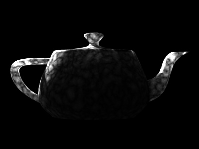
Let us now revisit the teapot example from the previous sections, but set the diffuse mean free path very short:
Surface "render_ssdiffusion" "filename" "direct_rad_t.ptc"
  # Albedo for apple, but mean free path 1/10th of apple:
  "color albedo" [0.846 0.841 0.528]
  "color dmfp" [0.6961 0.6400 0.1896]   # very short mean free path!
  "float ior" 1.3
  "float smooth" 1
  "float maxsolidangle" 1.0
The subsurface scattering image looks like this with "smooth" 0 and 1, respectively:
With "smooth" 0 |
With "smooth" 1 |
ptfilter has a similar new smoothing functionality. It is turned on by specifying -smooth 1 on the command line.
5 Avoiding scattering across concavities
In PRMan 15.2 (and later versions) it is possible to reduce subsurface scattering across local concavities such as wrinkles, skin pores, lips, etc. This is done by setting the optional parameter "followtopology" to 1.0. The default is 0.0. Values between 0.0 and 1.0 results in partially reduced scattering across concavities.
ptfilter has a similar new functionality; it is turned on by specifying ``-followtopology f (with f being a value between 0.0 and 1.0) on the command line.
6 Ray-traced subsurface scattering
In release 16.2 we added a ray-traced mode for subsurface scattering. The scattering surface parameters, formulas and results are the same as for point-based subsurface scattering. However, the biggest advantage of the ray-traced approach is that it is single-pass - no need to bake a point cloud in a pre-pass. This makes it particularly suitable for interactive rendering and re-rendering.
When computing ray-traced subsurface scattering at a point P, the subsurface() function shoots a bunch of rays (in all directions on the sphere) originating from a point slightly inside the surface. This gives dense hitpoints near P and sparser hitpoints further away. The direct illumination at each hitpoint (on the outside of the object) is computed or retrieved from the radiosity cache and then attenuated by the usual dipole formula (the same formula as for point-based calculations).
The subsurface() function has an optional first parameter, "mode", which can be either "pointbased" (the default) or "raytraced". In raytraced mode, there are four new parameters:
- "samples": the number of rays. The default is 16.
- "offset": how far inside the surface to shoot the sss rays from. The default value is the min of two values: 1) the max of the three dmfp values, 2) half the object thickness at that point - this ensures that the sss rays aren't shot from beyond the backside of very thin objects. (In releases prior to PRMan 16.6 the default value was computed using the min rather than the max of the three dmfp values. Using the max gives less noise.)
- "subset": the subset of objects visible to sss rays. The default subset is the entire scene.
- "maxdist": the maximum distance for ray hits.
To use the ray-traced subsurface() function, a shader must be structured using the pipeline methods discussed in the Physically Plausible シェーディング in RSL application note. Since subsurface scattering is a view-independent part of an object's appearance, we will need to modify the lighting() and diffuselighting() methods.
The lighting() method is not required, but if your shader has one, call subsurface() instead of computing diffuse illumination.
public void lighting(output color Ci, Oi)
{
    initDiff();
    initSpec();

    color sss, spec;

    // Compute direct and indirect specular

    directlighting(this, m_lights, "specularresult", spec);

    spec += indirectspecular(this, "samplebase", 1,
                             "subset", indirectSpecularSubset,
                             "maxdist", specularMaxDistance);

    // Do *not* compute direct and indirect diffuse -- subsurface
    // handles those !!

    sss = subsurface("raytraced", P, m_shadingCtx->m_Nn,
                     "type", sssType,
                     "albedo", m_diffuse->m_diffカラー,
                     "diffusemeanfreepath", sssDMFP,
                     "ior", ior, "unitlength", sssUnitLength,
                     "samples", sssSamples, "maxdist", sssMaxDistance,
                     "offset", sssOffset);

    Ci = sss * m_fres->m_Kt + spec; // fresnel already in spec
}
The diffuselighting() method is required for ray-traced subsurface to operate properly. There is a new (optional) third parameter that must be filled with irradiance. Irradiance is the cosine-weighted sum of all direct lighting plus indirect diffuse lighting. If your shader implements its own light integration scheme, simply assign the proper value to the irradiance. Alternatively, the directlighting() integrator provided by RSL will compute the direct portion of irradiance as a side effect of computing direct lighting, returned in the optional output "irradianceresult". If indirectdiffuse() is employed by the shader, it should be accumulated into the irradiance.
public void diffuselighting(output color Ci, Oi, Ii)
{
    initDiff();

    string raylabel;
    rayinfo("label", raylabel);

    if (raylabel == "subsurface") {

        // Compute direct diffuse and irradiance.
        directlighting(this, m_lights,
                       "diffuseresult", Ci,
                       "irradianceresult", Ii);
        // Divide directlighting() irradianceresult Ii by pi (similar to
        // what directlighting() does internally for diffuse: mult by
        // albedo / pi).
        Ii *= 1/PI;

        // Compute indirect diffuse and irradiance.
        if (indirectDiffuseSamples > 0) {
            color indirect = indirectdiffuse(P, m_shadingCtx->m_Ns,
                                    m_indirectSamples, "adaptive", 1,
                                    "maxvariation", indirectDiffuseMaxVar,
                                    "maxdist", indirectDiffuseMaxDistance);
            Ci += m_diffuse->m_diffカラー * indirect;
            Ii += indirect;
        }

    } else {

        Ci = subsurface("raytraced", P, m_shadingCtx->m_Nn,
                        "type", sssType,
                        "albedo", m_diffuse->m_diffカラー,
                        "diffusemeanfreepath", sssDMFP,
                        "ior", ior, "unitlength", sssUnitLength,
                        "samples", sssSamples, "maxdist", sssMaxDistance,
                        "offset", sss_offset);
    }
}
Note the assignment of irradiance (without surface scattering) to the new output variable Irradiance.
These two short shader examples leave out some optimizations that are important in actual use: reduction of the sample numbers at deeper ray depths, optionally turning off indirect diffuse at subsurface ray hits, and optionally turning off subsurface scattering at diffuse ray hits. The plausibleSubSurface shader is a more complete shader example with these optimizations.
In this shader, the surface albedo is ignored where the illumination enters the surface; it is only taken into account where the subsurface illum leaves the surface (the shading point). An alternative is to use the albedo where the subsurface illum enter the surface but ignore it where it leaves, or use the square root of the albedo both places. It would be wrong to use the full albedo both where the light enters the surface and where it leaves it; this leads to too dark and saturated subsurface scattering results.
Known caveat: ray-traced subsurface scattering does not work with double-shading. (This is because the subsurface calculations need to know the non-flipped normal when computing direct illumination.)
In release 17.0 we added a way to access the Irradiance output value by fetching it with the gather() "lighting:irradianceoutside" output variable. The value is denoted as outside because the I vector at the hit point is set as if the gather was from the outside for shading purposes. This means it will fetch the outside irradiance, making it suitable for implementing single scattering or creating custom subsurface integrators. The renderer can cache the Irradiance value, providing better performance than fetching the irradiance from an arbitrary shader output parameter.
When fetching "lighting:irradianceoutside", the diffuse and specular depths remain the same at hit points. The subsurface depth is increased, which can be accessed via a rayinfo() query of "subsurfacedepth".
float ssdepth, irrad;
rayinfo("subsurfacedepth",ssdepth);
if (ssdepth == 0 ) {
   gather("illuminance", Pinside, Nn, blur, samples,
          "lighting:irradianceoutside", irrad) {
     ...
    }
}
Currently, we disallow fetching "lighting:irradianceoutside" with output values other than "primitive:P," "primitive:N," and "ray:" queries in the same gather() call. Sending values with the rays is still permitted.
7 Single scattering
Single scattering is not important in materials such as skin. For other materials where it is more important it can be done in a shader using the trace() and transmission() functions.
8 No scattering (absorption only)
Another effect that occurs in participating media is that some of the light from the surfaces travels straight through the medium without being scattered. Due to absorption, the amount of light that is transported this way falls off exponentially with the distance through the medium.
An object of frosted, colored glass is a good example of this type of light transport. The frosted surface of the glass scatters the light diffusely into the object. The internal part of the glass is clear and scatters very little light (but absorbs some of the light due to the coloring).
This effect can be computed by shooting rays with the gather() construct. Basically, for each visible shading point, we want to shoot a collection of rays from that point into the object and look up the direct illumination at the surface points those rays hit.
So the shader needs to distinguish between whether it is running on a directly visible point or on a subsurface ray hit point. A ray label is used to communicate this information.
It is assumed that the surfaces have the correct orientation, i.e. that the normals are pointing out of the objects.
8.1 Baking direct illumination
We first compute the direct illumination and store it just as in Section 2.1.
8.2 Creating a brick map
We need to convert the point cloud direct_rad_t.ptc (representing direct illumination transmitted through the surface) to a brick map so that the texture3d() function can read it efficiently. This is done with the brickmake program:
brickmake -maxerror 0.002 direct_rad_t.ptc direct_rad_t.bkm
The brick map can be displayed using the brickviewer program.
8.3 レンダリング
A shader that renders light transmission with absorption (and direct illumination if so desired) with the help of a brick map of the direct illumination is listed below. The shader utilizes the convention that if the texture3d() call fails to find the requested value, it does not change the value of the rad_t parameter. So in this shader, we can get away with not checking the return code of texture3d(): if it fails, rad_t will remain black.
surface
subsurf_noscatter(float Ka = 1, Kd = 1, Ks = 1, roughness = 0.1;
                  float Ksub = 1, extcoeff = 1, samples = 16;
                  string filename = "")
{
    color rad_t = 0;
    normal Nn = normalize(N);
    vector Vn = -normalize(I);
    uniform string raylabel;

    rayinfo("label", raylabel);

    if (raylabel == "subsurface") { /* subsurface ray from inside object */

        /* Lookup precomputed irradiance (use black if none found) */
        texture3d(filename, P, Nn, "_radiance_t", rad_t);
        Ci = rad_t;

    } else { /* regular shading (from outside object) */

        color raycolor = 0, sum = 0, irrad;
        float dist = 0;

        /* Compute direct illumination (ambient, diffuse, specular) */
        Ci = (Ka*ambient() + Kd*diffuse(Nn)) * Cs
             + Ks*specular(Nn,Vn,roughness);

        /* Add transmitted light */
        if (Ksub > 0) {
            gather("illuminance", P, -Nn, PI/2, samples,
                   "label", "subsurface",
                   "surface:Ci", raycolor, "ray:length", dist) {
                sum += exp(-extcoeff*dist) * raycolor;
            }
            irrad = sum / samples;
            Ci += Ksub * irrad * Cs;
        }
    }

    Ci *= Os;
    Oi = Os;
}
The image below shows the resulting light transmission through a teapot:
Teapot with light transmission
レンダリング this image requires 6.3 million subsurface rays, so it is significantly slower than computing the diffusion approximation in Section 2.
9 Frequently Asked Questions
Q: Which method does ptfilter use to compute subsurface scattering?
A: We use the efficient hierarchical diffusion approximation by Jensen and co-authors - see the references below.
Q: If I specify the material for the diffusion simulation, how can I get to see the corresponding material parameters that are being used in the simulation?
A: Use the -progress 1 or -progress 2 flag for ptfilter. This prints out various information during the simulation calculation.
Q: I see banding in the subsurface scattering (diffusion) result produced by ptfilter. How can I get rid of the bands?
A: Decrease the maxsolidangle in ptfilter and/or increase the density of baked points (for example by decreasing the shadingrate or increasing the image resolution).
Q: The ptfilter diffusion computation is too slow. How can I speed it up?
A: Increase the maxsolidangle in ptfilter and/or decrease the number of baked points (for example by increasing shadingrate or decreasing image resolution). And/or run ptfilter multithreaded with -threads n.
Q: The brick map generated by brickmake is huge. How can I make it smaller?
A: Use maxerror values of 0.002, 0.004, or 0.01 (or even higher) in brickmake.
Q: What exactly is the maxsolidangle parameter of ptfilter's diffusion approximation?
A: maxsolidangle is the parameter called epsilon on page 579 of [Jensen02].
Q: Computing subsurface scattering with the subsurface() function seems to take longer than when I use ptfilter. Is that expected?
A: The same algorithm is used for the subsurface() function as for ptfilter's ssdiffusion calculation. So given the same input parameters and number of computation points, the computation times will be the same. However, if the value of e.g. "maxsolidangle" differs, the computation times will differ as well. In addition, if there are more shading points running the subsurface() function than there are points in the point cloud that ptfilter is run on, the calculations are done more times in the former case, and the computation time will be longer.
Q: The channels in my input point cloud are not called "_area" and "_radiance_t". How can I get subsurface() or ptfilter to read the data from channels with a different name?
A: For the subsurface() function, the channel names can be specified with the "areachannel" and "radiancechannel" parameters. For ptfilter -ssdiffusion, use the command line options -areachannel and -radiancechannel.
Q: The point-based subsurface scattering results look splotchy. What can I do?
A: The point cloud file may be too sparse relative to the mean free path length of light in the material. As a rule of thumb, the max distance between points in the point cloud should be the mean free path. However, even in this challenging situation, smooth results can be obtained by setting the subsurface() function parameter "smooth" to 1, or use the ptfilter command line option -smooth 1.
10 Improvements and extensions
First of all, the illumination on the surface of the examples is purely direct illumination. It could just as well be high dynamic range illumination from an environment map or global illumination taking indirect illumination of the teapot into account.
Second, the 3D texture is only evaluated on the surfaces. In order to improve the accuracy of light extinction inside the object the 3D texture should be evaluated inside the object, too. This requires evaluation of the 3D texture at many positions along each subsurface ray.
More information about the methods we use for efficient simulation of subsurface scattering can be found in the following publications:
[Jensen01] Henrik Wann Jensen, Stephen R. Marschner, Marc Levoy, and Pat Hanrahan. A Practical Model for Subsurface Light Transport. Proceedings of SIGGRAPH 2001, pages 511-518.
[Jensen02] Henrik Wann Jensen and Juan Buhler. A Rapid Hierarchical レンダリング Technique for Translucent マテリアル. Proceedings of SIGGRAPH 2002, pages 576-581.
[Hery03] Christophe Hery. Implementing a Skin BSSRDF. In "RenderMan, Theory and Practice", SIGGRAPH 2003 Course Note #9, pages 73-88.
The topology-dependent diminishing in locally concave areas is inspired by this course note:
Erin Tomson. Human Skin for "Finding Nemo". In "RenderMan, Theory and Practice," SIGGRAPH 2003 Course Note #9, page 90.
The smooth parameter is inspired by this poster:
Anders Langlands and Tom Mertens. Noise-Free BSSRDF レンダリング On The Cheap. SIGGRAPH 2007 Poster.
An interesting alternative to the dipole approximation is described in this paper:
Eugene d'Eon and Geoffrey Irving. A Quantized-Diffusion Model for レンダリング Translucent マテリアル. Proceedings of SIGGRAPH 2011, article 56.
Information about PRMan's ray tracing functionality can be found in the application note "A Tour of Ray-Traced シェーディング in PRMan". More information about point clouds and brick maps can be found in application note "Baking 3D テクスチャs: Point Clouds and Brick Maps".
The source code of our implementation of subsurface scattering is listed as an example in Section 1.3 of "The Point Cloud File API".