Baking 3D テクスチャs
Baking 3D テクスチャs
Point Clouds and Brick Maps
May, 2004 (Revised: November, 2010)
- 1 Introduction
- 2 Baking data as point clouds
- 3 Reading point cloud files
- 4 Organized point clouds
- 5 Brick maps
- 5.1 What is a brick map?
- 5.2 Advantages of the brick map representation
- 5.3 Creating a brick map from a point cloud
- 5.4 Displaying a brick map
- 5.5 Reading data from a brick map
- 5.6 Raw brick map data
- 5.7 フィルタリング, blur, and lerp
- 5.8 Brick cache size
- 5.9 Limiting the number of open files
- 5.10 Brick maps and incoherent normals
- 6 Baking and reading volume data
- 7 Caching of data
- 8 The getpoints() function
- 9 Common pitfalls and known issues
- 10 Frequently asked questions
- 11 More information
1 Introduction
The purpose of this application note is to provide recipes and examples for baking and reusing general 3D textures in Pixar's RenderMan (PRMan). The approach described herein is general and can be used to bake data such as diffuse color, highlights, direct and indirect illumination, ambient occlusion, etc.
The primary example used below is baking light from an area light source; the light illuminates a simple scene consisting of a cylinder and a plane. Since the soft shadows from an area light source are rather slow to compute, it is appealing to compute and bake it only once and then reuse it for many subsequent renderings. In another example, we bake illuminated surface colors.
2 Baking data as point clouds
Arbitrary 3D data can be written to a file ("baked") with the bake3d function. Here is an example of the syntax:
bake3d(filename, displaychannels, P, N, "radius", r, "coordsystem", cs,
       "interpolate", 0,
       "direct", d, "onebounce", ob, "occlusion", occ, ... );
The displaychannels parameter is a string consisting of a comma-separated list of channel names. Each channel name must be specified in the RIB file.
For example:
DisplayChannel "color direct"
DisplayChannel "color onebounce"
DisplayChannel "float occlusion"
The corresponding displaychannels is the string "direct,onebounce,occlusion".
If N is (0, 0, 0) the data points are considered spheres instead of oriented disks.
When the optional parameter "radius" is omitted, PRMan automatically computes a radius that corresponds to the size of a shading micropolygon. If the radius is set to 0, the data are considered infinitely small points instead of disks (or spheres).
When "interpolate" is 0, the actual points P are baked. This can result in "overlapping" points at shading grid edges. If "interpolate" is 1, the point positions, normals, radii, and data are interpolated from four shading points. This can be used to bake out micropolygon midpoints rather than the actual shading points, to avoid overlapping points at shading grid edges.
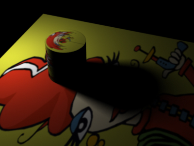
2.1 Example: baking surface illumination
In this example, we'll bake the illumination from a pseudo area light source shining onto a couple of objects. The area light source shader uses a lot of ray tracing to compute the soft shadows, so it is relatively time-consuming, and hence it pays off to bake the illumination. The area light source shader is "spherelight" which is a standard shader distributed with PRMan. The surface shader looks like this:
surface
bake_direct_irrad(string filename = "", displaychannels = "";
                  float interpolate = 1)
{
    color irrad;
    normal Nn = normalize(N);

    /* Compute direct illumination (ambient and diffuse) */
    irrad = ambient() + diffuse(Nn);

    /* Store in point cloud file */
    bake3d(filename, displaychannels, P, Nn, "interpolate", interpolate,
           "_irradiance", irrad);

    Ci = irrad * Cs * Os;
    Oi = Os;
}
The RIB file looks like this:
FrameBegin 0

  Format 400 300 1
  シェーディングInterpolation "smooth"
  PixelSamples 4 4

  Display "bake_arealight" "it" "rgba"
  Quantize "rgba" 255 0 255 0.5
  DisplayChannel "color _irradiance"

  Projection "perspective" "fov" 25
  Translate 0 -0.5 8
  Rotate -40  1 0 0
  Rotate 20  0 1 0

  Attribute "trace" "bias" 0.0001

  WorldBegin

    Attribute "cull" "hidden" 0   # don't cull hidden surfaces
    Attribute "cull" "backfacing" 0   # don't cull backfacing surfaces
    Attribute "dice" "rasterorient" 0   # view-independent dicing !
    Attribute "visibility" "int diffuse" 1   # make objects visible to rays
    Attribute "visibility" "int specular" 1   # make objects visible to rays

    LightSource "spherelight" 1 "from" [-2.8 2 0.5] "radius" 0.2
      "intensity" 2 "samples" 64 "falloff" 1

    Sides 1   # to avoid flipping normals in "spherelight"

    # Ground plane
    AttributeBegin
      Surface "bake_direct_irrad" "filename" "area_illum_plane.ptc"
        "displaychannels" "_irradiance"
      Scale 3 3 3
      Polygon "P" [ -1 0 1  1 0 1  1 0 -1  -1 0 -1 ]
    AttributeEnd

    Attribute "visibility" "int transmission" 1 # the cyl. casts shadow
    Attribute "shade" "transmissionhitmode" "primitive"

    # Cylinder with cap
    AttributeBegin
      Surface "bake_direct_irrad" "filename" "area_illum_cyl.ptc"
        "displaychannels" "_irradiance"
      Translate -1 0 0.5
      Rotate -90 1 0 0
      Cylinder 0.5 0 1 360
      Disk 1 0.5 360
    AttributeEnd

  WorldEnd
FrameEnd
Running this RIB file renders the following image:
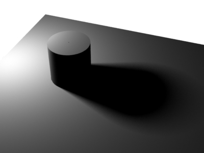
Baked direct illumination values (with soft shadow)
It also generates two point cloud files: area_illum_plane.ptc and area_illum_cyl.ptc. The point cloud files can be displayed with the ptviewer program.
area_illum_plane.ptc |
area_illum_cyl.ptc |
These two point cloud files contain 170,000 points and 31,000 points and take up 5.4 MB and 1 MB, respectively. (If "interpolate" is set to 0 in the bake3d() call, the resulting point cloud files contain 200,000 and 36,000 points.) The number of points generated can be adjusted by changing either the shading rate or the image resolution.
2.2 Example: baking illuminated surface colors
The next example is more colorful. Here we bake the illuminated surface colors, i.e. the product of the illumination and surface color. The light source shader is the same as before, but the surface shader now looks like this:
surface
bake_illumsurfcolor(string filename = "", displaychannels = "", texturename = "";
                    float interpolate = 1)
{
    color irrad, tex = 1, illumsurfcolor;
    normal Nn = normalize(N);

    /* Compute direct illumination (ambient and diffuse) */
    irrad = ambient() + diffuse(Nn);

    /* Multiply by surface color */
    if (texturename != "")
        tex = texture(texturename);
    illumsurfcolor = irrad * tex * Cs;

    /* Store in point cloud file */
    bake3d(filename, displaychannels, P, Nn, "interpolate", interpolate,
           "_illumsurfcolor", illumsurfcolor);

    Ci = illumsurfcolor * Os;
    Oi = Os;
}
The RIB file is similar to the previous example, but with a few related changes to the surfaces:
FrameBegin 0

  Format 400 300 1
  シェーディングInterpolation "smooth"
  PixelSamples 4 4

  Display "bake_illumsurf" "it" "rgba"
  Quantize "rgba" 255 0 255 0.5
  DisplayChannel "color _illumsurfcolor"

  Projection "perspective" "fov" 25
  Translate 0 -0.5 8
  Rotate -40  1 0 0
  Rotate 20  0 1 0

  Attribute "trace" "bias" 0.0001

  WorldBegin

    Attribute "cull" "hidden" 0   # don't cull hidden surfaces
    Attribute "cull" "backfacing" 0   # don't cull backfacing surfaces
    Attribute "dice" "rasterorient" 0   # view-independent dicing !
    Attribute "visibility" "int diffuse" 1   # make objects visible to rays
    Attribute "visibility" "int specular" 1   # make objects visible to rays

    LightSource "spherelight" 1 "from" [-2.8 2 0.5] "radius" 0.2
      "intensity" 2 "samples" 64 "falloff" 1

    Sides 1   # to avoid flipping normals in "spherelight"

    # Ground plane
    AttributeBegin
      Surface "bake_illumsurfcolor" "filename" "illumsurf_plane.ptc"
        "displaychannels" "_illumsurfcolor" "texturename" "irma.tex"
      Scale 3 3 3
      Polygon "P" [ -1 0 1  1 0 1  1 0 -1  -1 0 -1 ]
      "s" [1 1 0 0]
      "t" [0 1 1 0]
    AttributeEnd

    Attribute "visibility" "int transmission" 1 # the cyl. casts shadow
    Attribute "shade" "transmissionhitmode" "primitive"

    # Cylinder with cap
    AttributeBegin
      Surface "bake_illumsurfcolor" "filename" "illumsurf_cyl.ptc"
        "displaychannels" "_illumsurfcolor" "texturename" "irma.tex"
      Translate -1 0 0.5
      Rotate -90 1 0 0
      Cylinder 0.5 1 0 -360   # reversed to get texture right side up
      Disk 1 0.5 360
    AttributeEnd

  WorldEnd
FrameEnd
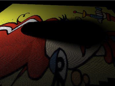
Running this RIB file renders the following image and point clouds:

Baked illuminated surface colors
illumsurf_plane.ptc |
illumsurf_cyl.ptc |
As in the previous example, the point cloud files contain 170,000 points and 31,000 points, respectively. In these examples, we have chosen to bake into a separate point cloud for for each object. We could also have chosen to bake all points into a single point cloud file.
2.3 Baking and ray tracing
Shaders execute at the ray hit points if ray tracing is used to compute reflections, refractions, semitransparent shadows, or soft indirect illumination. If the shader calls bake3d() at those hit points (in addition to the regular REYES grid shading points), the point cloud will end up with both regularly spaced points from the REYES shading grids and irregularly scattered points from ray hits. Depending on the curvature of the geometry that shoots the rays, the data points from ray hits will have very different radius values associated with them, and their radii will also be very different from the data points from REYES grids on the same surface.
For some applications, this mix of data points with inconsistent radius values is harmless - or even desirable. However, in most cases we would like to bake data only from the REYES shading grid points. Here is a common and useful idiom to ensure this:
uniform float raydepth = 0;

rayinfo("depth", raydepth);

// Only bake data at REYES grid points; not at ray hit points
if (raydepth == 0) {
  bake3d(filename, displaychannels, P, Ns, ...);
}
This precaution is particularly important if we intend to use the point cloud to generate a brick map (as discussed in section 4) since brick map construction works best for point clouds with data points that are regularly spaced and with consistent radii.
3 Reading point cloud files
After the point cloud is generated, we can read it with the texture3d() function. Syntax example:
ok = texture3d(filename, P, N, "coordsystem", cs,
               "direct", d, "onebounce", ob, "occlusion", occ, ... );
If N is (0,0,0), the normals associated with the data points are ignored for the lookups.
3.1 Example: reading baked illuminated surface colors
In this example we read the illuminated surface colors from the point clouds generated in example in Section 2.2. Here is the surface shader:
surface
read_illumsurfcolor(uniform string filename = "")
{
    color illumsurfcolor = 0;
    normal Nn = normalize(N);
    float ok;

    ok = texture3d(filename, P, Nn, "_illumsurfcolor", illumsurfcolor);

    Ci = illumsurfcolor * Os;
    Oi = Os;
}
The RIB file is the same as when baking, but with a different surface shader, no light source, and no attributes for culling or dicing:
FrameBegin 0

  Format 400 300 1
  シェーディングInterpolation "smooth"
  PixelSamples 4 4

  Display "read_illumsurf" "it" "rgba"
  Quantize "rgba" 255 0 255 0.5

  Projection "perspective" "fov" 25
  Translate 0 -0.5 8
  Rotate -40  1 0 0
  Rotate 20  0 1 0

  WorldBegin

    # Ground plane
    AttributeBegin
      Surface "read_illumsurfcolor" "filename" "illumsurf_plane.ptc"
      Scale 3 3 3
      Polygon "P" [ -1 0 1  1 0 1  1 0 -1  -1 0 -1 ]
    AttributeEnd

    # Cylinder with cap
    AttributeBegin
      Surface "read_illumsurfcolor" "filename" "illumsurf_cyl.ptc"
      Translate -1 0 0.5
      Rotate -90 1 0 0
      Cylinder 0.5 0 1 360
      Disk 1 0.5 360
    AttributeEnd

  WorldEnd
FrameEnd
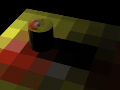
The resulting image looks like this:
Illuminated surface colors from point cloud lookups
レンダリング this image is very fast, and it is nearly identical to the image rendered during baking.
3.2 Drawbacks of reading point clouds
Unfortunately, reading unorganized point cloud files directly has several drawbacks:
- When an unorganized point cloud is accessed the entire point cloud file is read in - even if only a few points are used.
- The entire point cloud stays in memory until the frame has finished.
- The point cloud format does not provide a level-of-detail representation, making filtering and blurring difficult.
To overcome these limitations, we use two other data formats: organized point clouds and brick maps.
4 Organized point clouds
With standard point clouds, the entire point cloud has to be read in by texture3d() and all the points stay in memory until the frame is rendered to completion. In order to handle large point clouds more efficiently, RenderMan Pro Server 14.0 introduced a new file format: organized point cloud.
4.1 What is an organized point cloud?
An organized point cloud is a collection of data points organized into an octree. (The octree nodes can have additional data associated with them or not, depending on the application.)
4.2 Creating an organized point cloud
Use the ptfilter program with no filter but -organize 1 to generate an organized point cloud. For example:
ptfilter -organize 1 inputfiles.ptc outputfile.optc
Or even simpler:
ptfilter inputfiles.ptc outputfile.optc
Note
We recommend, but do not require, using the .optc suffix for organized point clouds.
The organized points can be displayed with ptviewer, and information about the number of nodes and their data types can be obtained with ptviewer -info or -onlyinfo. The point cloud is organized if the listed number of tree nodes is larger than zero.
4.3 Reading an organized point cloud
The texture3d() function reads the points and octree nodes from an organized point cloud on demand, and caches them in a fixed-size cache. An organized point cloud is passed to texture3d() with the filename parameter (just like unorganized point clouds). The difference is that texture3d() can lookup texture data in an organized point clouds without loading the entire point cloud.
Known limitation: texture3d() can't handle gzipped organized point cloud files (but it can read gzipped unorganized point cloud files without problems.) If texture3d() reads a gzipped organized point cloud, a warning message will be printed, and the point cloud will be treated as if it were unorganized.
4.4 Cache sizes
When points and octree nodes are read by texture3d() they are stored in caches. This makes it possible to efficiently read data from very large organized point cloud files.
The default size of the caches is 10 MB, but it can be controlled with Option "limits" "pointmemory" and Option "limits" "octreememory". The size is specified in kB, so to specify two 50 MB caches, use:
Option "limits" "pointmemory" 51200
Option "limits" "octreememory" 51200
Alternatively, the cache sizes can be specified in the rendermn.ini file, thusly:
/prman/pointmemory          51200
/prman/octreememory         51200
As usual, the Option overrides the rendermn.ini setting if both are used.
However, the specified cache sizes are only used as a guideline. The number of cache entries is determined by the cache size and the number of data per point in the first point read. If any of the following points have more data, the point cache entries will be enlarged on-the-fly, and the end result is a cache using more memory than specified by the option (or rendermn.ini file). This also applies to the octree cache. To further confuse the issue, in multithreaded execution there are caches for each thread, so the total cache size increases as more threads are used.
Sometimes increasing the cache sizes can speed up rendering significantly. You can determine if this is might be worthwhile to try by inspecting the statistics under the point/octreeCache tab. The first warning sign is if a significant part of the overall render time is spent in system calls (reading points and octree nodes from disk). The second warning sign is if the cache miss rates (e.g. Point cache misses / Point cache lookups) is above a few percent. (Due to compulsory cache misses, the rate will never reach 0 no matter how large the cache is.) If these warning signs are seen, there is a good chance that increasing one or both cache sizes will speed up rendering.
5 Brick maps
In order to facilitate efficient rendering of large sets of baked data it is necessary to convert the unordered point clouds to a MIP map representation suitable for efficient filtering and caching. We use brick maps for this.
5.1 What is a brick map?
A brick map is an adaptive, sparse octree with a brick at each octree node. A brick is a 3D generalization of a texture tile; each brick consists of 8^3 voxels with (possibly sparse) data values. The data can be colors, such as diffuse color, specular color, illumination, shadow, etc., and/or floats, such as ambient occlusion, etc. The brick map format is a 3D generalization of Pixar's tiled 2D MIP map texture format for normal 2D textures.
The images below show three levels of a sparse brick map for surface data:
Level 0 |
Level 1 |
Level 2 |
The images below show three levels of a dense brick map for volume data:
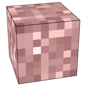
Level 0 |
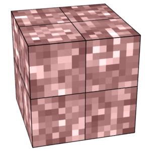
Level 1 |
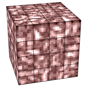
Level 2 |
5.2 Advantages of the brick map representation
The brick map format has several advantages:
- The brick map is independent of the surface representation.
- No 2D surface parameterization is necessary. (Specifying a 2D parameterization for surfaces such as subdivision surfaces, implicit surfaces, and dense polygon meshes can be cumbersome.)
- Brick maps automatically adapt to the data density and variation. If, for example, a fairly smooth 3D texture has only one small region with a lot of detail, there will only be many bricks in that one small region. (This is in contrast to traditional 2D textures where the entire texture has to have high resolution if just a small part of it has a lot of detail.)
- The MIP map representation is suitable for efficient filtering, and the tiling makes it ideal for caching. This means that PRMan can deal efficiently with large brick maps - even collections of brick maps much larger than the available memory.
- The user can specify the required accuracy when the brick map is created. This makes it simple to trade off data precision vs. file size.
5.3 Creating a brick map from a point cloud
A brick map is created from a point cloud using brickmake. The syntax is:
brickmake [-maxerror eps] [-maxdepth md] pointcloudfile(s) brickmapfile
For example:
brickmake -maxerror 0.002 illumsurf_plane.ptc illumsurf_plane.bkm
brickmake -maxerror 0.002 illumsurf_cyl.ptc illumsurf_cyl.bkm
For this example, the resulting brick maps contain approximately 4100 and 1700 bricks and use 2.8 MB and 1.3 MB, respectively.
Maxerror is a trade-off between precision and file size. Using a negative value for maxerror means that no data will be reduced/compressed. For very small values of maxerror (for example 0.0001) only very uniform data (as on the black side of the cylinder) will be compressed. The default value for maxerror is 0.002 which corresponds roughly to half of 1/255. Maxerror values of 0.001 to 0.01 are good to use in practice for data values in the [0,1] range.
Maxdepth specifies the maximum depth of the brick map octree. The default value is 15, which usually has no effect.
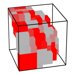
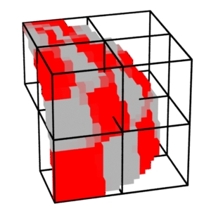
5.4 Displaying a brick map
Brick maps can be displayed with the interactive viewing program brickviewer. For example, to display the cylinder brick map, type:
brickviewer illumsurf_cyl.bkm
Here are a couple of screen shots of brickviewer in action. Both images show level 1 of the cylinder brick map. The left image shows the default display mode, where the faces of each voxel are shown. The right image shows the fast display mode where each voxel is shown as one square facing the screen.
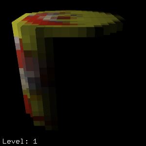
Nice display mode (default) |
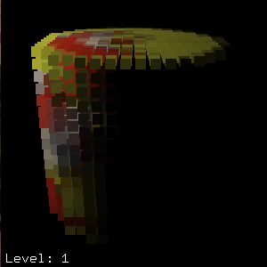
Fast display mode |
Brickviewer is controlled with the following keys:
- s switches between fast (approximate) and nice ("slow&") display mode.
- up/down arrows switch level.
- left/right arrows adjust point size in approximate mode.
- t toggles fps display.
5.5 Reading data from a brick map
Arbitrary 3D data in brick map format can be read in with the texture3d() function. Here is an example of the syntax:
ok = texture3d(filename, P, N, "filterradius", r, "coordsystem", cs,
               "direct", d, "onebounce", ob, "occlusion", occ, ... );
When the optional parameter "filterradius" is omitted, PRMan will automatically compute a filter radius that corresponds to the size of a shading micropolygon or the finest resolution in the brick map, whichever is largest.
The variables can be read in a different order than the order they were baked in. It is also possible to read only a subset of the baked variables.
Example: reading baked illuminated surface colors
In this example we read the brick map generated in the previous section. The surface shader is the same as in Section 3.1. The RIB file is also the same as in Section 3.1, but with the point cloud file names replaced by the brick map file names:
FrameBegin 0

  Format 400 300 1
  シェーディングInterpolation "smooth"
  PixelSamples 4 4

  Display "read_illumsurf" "it" "rgba"
  Quantize "rgba" 255 0 255 0.5

  Projection "perspective" "fov" 25
  Translate 0 -0.5 8
  Rotate -40  1 0 0
  Rotate 20  0 1 0

  WorldBegin

    # Ground plane
    AttributeBegin
      Surface "read_illumsurfcolor" "filename" "illumsurf_plane.bkm"
      Scale 3 3 3
      Polygon "P" [ -1 0 1  1 0 1  1 0 -1  -1 0 -1 ]
    AttributeEnd

    # Cylinder with cap
    AttributeBegin
      Surface "read_illumsurfcolor" "filename" "illumsurf_cyl.bkm"
      Translate -1 0 0.5
      Rotate -90 1 0 0
      Cylinder 0.5 0 1 360
      Disk 1 0.5 360
    AttributeEnd

  WorldEnd
FrameEnd
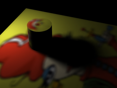
The resulting image looks like this:

Illuminated surface colors from brick map lookups
レンダリング this image takes less than 10 seconds. It is nearly identical to the image rendered during baking.
5.6 Raw brick map data
If, out of curiosity, we are interested in rendering the raw, uninterpolated brick map data, we can set "filterradius" to 0 in the texture3d() calls. The rendered image looks like this:

Lookups with filterradius 0
Upon close inspection it is possible to make out the individual large voxels in regions with smooth color variation. As another example, in the image below the brick maps have been generated with maxerror 0.02 to make the voxels clearer. (These brick maps still contain approximately 4100 and 1700 bricks, but now use only 1.2 MB and 0.8 MB, respectively.)

Lookups with filterradius 0 (brickmake maxerror 0.02)
Notice that the voxels are large in areas with uniform color and small in regions with sharp details.
The texture3d() parameter "maxdepth" can be used to render using only the top levels of the brick map. The images below are rendered with "filterradius" 0 and "maxdepth" 0 and 1, respectively:
Lookups with filterradius 0 and maxdepth 0 |

Lookups with filterradius 0 and maxdepth 1 |
5.7 フィルタリング, blur, and lerp
As mentioned previously, PRMan will automatically compute a filter radius that corresponds to the area of a micropolygon (or the finest resolution in the brick map). But the filterradius can also be explicitly set in order to blur the lookup results. Filterradius is measured in world space units. The images below show two examples corresponding to "filtersize" 0.03 and 0.1.

Lookups with filterradius 0.03 |

Lookups with filterradius 0.1 |
It is interesting to note that, although the textures are blurred in most regions, the color contrast across the sharp edge of the cylinder is still sharp. This is because the brick map data are stored in separate octrees depending on the orientation.
Another way of specifying the filter radius is as a multiple of the micropolygon size. If the filterradius is not specified, filterradius values corresponding to the size of the micropolygons are automatically computed. This means that each texture3d() result corresponds to the average texture over the area of the micropolygon. The optional parameter "filterscale" can be used to scale this default filter size; the images below show some examples:

Lookups with filterscale 1 (the default) |

Lookups with filterscale 3 |

Lookups with filterscale 5 |
Lookups with filterscale 10 |
In order to ensure smooth transitions between different lookups (for example in a zoom out of a scene), the lookups can be linearly interpolated between two levels in the brick map. This is specified by setting the optional parameter "lerp" to 1. The default is 0.
5.8 Brick cache size
When bricks are read by texture3d() they are stored in a cache. The size of the brick cache can be changed with Option "limits" "brickmemory". The size is specified in kB, so to specify a 10 MB cache, use
Option "limits" "brickmemory" 10240
The default brick cache size is 10 MB (same as above).
The brick cache size can also be specified in the rendermn.ini file. The syntax is as follows:
/prman/brickmemory 10240
As usual, the option overrides the .rendermn.ini setting if both are specified.
The specified brick cache size is only used as a guideline. The number of cache entries is determined by the cache size and the number of data pr. voxel in the first brick read in. If any of the following bricks have more data pr. voxel, the brick cache entries will be enlarged on-the-fly, and the end result is a brick cache using more memory than specified by the option (or rendermn.ini file). To further confuse the issue, in multithreaded execution there is a brick cache for each thread, so the total brick cache size increases the more threads are used.
Sometimes increasing the brick cache size can speed up rendering significantly. You can determine if this is might be a worthwhile endeavor by inspecting the statistics. The first warning sign is if a significant part of the overall render time is spent in system calls (reading bricks from disk). The second warning sign is if the brick cache capacity miss rate (ie. 'Capacity cache misses' / 'Brick cache lookups') is above a few percent. (The brick cache compulsory miss rate, 'Compulsory cache misses' / 'Brick cache lookups', is due to the first read of each brick, and that rate will not change no matter how large the cache is.) The third warning sign is if the 'brick read time' statistic is a large fraction of the overall render time. If all three warning signs are seen, there is a good chance that increasing the brick cache size will speed up rendering.
5.9 Limiting the number of open files
The maximum number of 3D texture files (brick maps and point clouds) that can be open simultaneously can be limited by a rendermn.ini setting:
/prman/texture3d/maxfiles 64
The default number is 64. When the number of open files exceeds this value, the least recently used file will be closed.
5.10 Brick maps and incoherent normals
Normals are disambiguated at all levels of the brick map. So it is perfectly fine to bake data from double-sided shading into a single brick map, and data can be looked up with wide filters without getting data that are mixed from front- and back-sides. The correct surface normal must be used, otherwise the lookups will fail.
6 Baking and reading volume data
In this section, we'll bake and lookup volume data: a smoke texture and volume illumination inside a cubic volume. When baking and looking up volume data it is important to use a "null" normal, i.e. N = (0,0,0), to distinguish the data from surface data.
6.1 Example: baking a 3D smoke texture
The following volume shader ray marches through a volume and computes a smoke density value at each step. It writes the values out to a point cloud file (as float data):
// Compute turbulent smoke density
float
smokedensity(point Pcurrent; float frequency, octaves)
{
  point Pshad = transform("shader", Pcurrent);
  point Psmoke = Pshad * frequency;

  // Compute smoke texture
  float smoke = 0, f = 1, i;
  for (i = 0; i < octaves; i += 1) {
    smoke += f * noise(Psmoke);
    f *= 0.5;
    Psmoke *= 2;
  }
  return smoke;
}

// Bake a volume full of smoke densities
volume
bakesmokevol(string filename = "", displaychannel = "";
             float frequency = 1, octaves = 3, depth = 1, steps = 100)
{
  point Pfront, Pcurrent;
  normal N0 = 0;
  vector In = normalize(I);
  vector dx = depth/steps * In, offset;
  float sd;
  uniform float step = 0;

  // Compute a start position (jittered in depth)
  Pfront = P - depth * In;
  offset = random() * dx;
  Pcurrent = Pfront + offset;

  // March along a ray through the volume
  while (step < steps) {

    // Compute the turbulent smoke density at Pcurrent
    sd = smokedensity(Pcurrent, frequency, octaves);

    // Write the 3D texture data point to a point cloud file
    bake3d(filename, displaychannel, Pcurrent, N0, "smokedensity", sd);

    // Advance one step
    step += 1;
    Pcurrent += dx;
  }

  // Use color from last step
  Ci = sd;
  Oi = 1;
}
In addition to writing the point cloud file, the shader also generates an image of the deepest slice of the smoke (the last assignment to Ci).
The following RIB file renders a 2x2x2 volume and bakes out a dense 3D point cloud file called smokevol.ptc.
FrameBegin 0

  Format 200 200 1
  シェーディングInterpolation "smooth"
  PixelSamples 4 4
  シェーディングRate 4

  Display "Baking volume texture data: smoke density" "it" "rgba"
  Quantize "rgba" 255 0 255 0.5
  DisplayChannel "float smokedensity"

  Projection "orthographic"
  Translate 0 0 10

  WorldBegin

    # Atmosphere shader bakes volume texture
    Atmosphere "bakesmokevol"
      "filename" "smokevol.ptc" "displaychannel" "smokedensity"
      "frequency" 5
      "depth" 2 "steps" 100

    # Back wall -- necessary to execute the atmosphere shader
    Surface "constant"
    Polygon "P" [-1 -1 1  1 -1 1  1 1 1  -1 1 1]

  WorldEnd
FrameEnd
Running this RIB file renders the following image. The image shows the smoke density at the back wall.
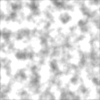
Baked 3D smoke texture
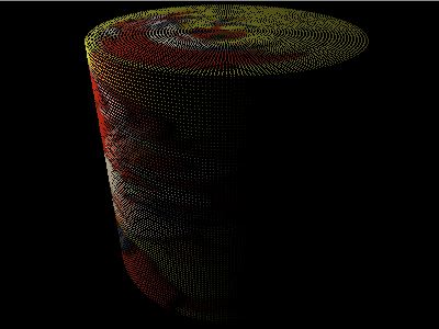
The baked point cloud, smokevol.ptc, has around 1.2 million data points (110x110x100). It is shown below:
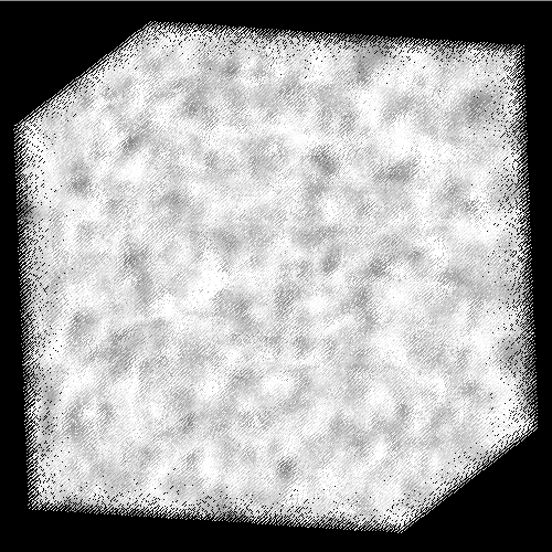
Point cloud of baked 3D smoke texture values
6.2 Example: baking volume illumination
In this example, we bake the illumination and shadow in a volume (again using ray marching). The illumination is stored as a color.
volume
bakeillumvol(string filename = "", displaychannel = "";
             float depth = 1, steps = 100)
{
  color li = 0;
  point Pfront, Pcurrent;
  normal N0 = 0;
  vector In = normalize(I);
  vector dx = depth/steps * In, offset;
  float smoke;
  uniform float step = 0;

  // Compute a start position (jittered in depth)
  Pfront = P - depth * In;
  offset = random() * dx;
  Pcurrent = Pfront + offset;

  // March along a ray through the volume
  while (step < steps) {

    // Compute the illumination (including shadows) at Pcurrent
    li = 0;
    illuminance(Pcurrent) {
      li += Cl;
    }

    // Write the illumination value to a point cloud file
    bake3d(filename, displaychannel, Pcurrent, N0, "illum", li);

    // Advance one step
    step += 1;
    Pcurrent += dx;
  }

  // Use color from last step
  Ci = li;
  Oi = 1;
}
The RIB file contains a spot light, a sphere casting a shadow, and a volume.
FrameBegin 0

  Format 200 200 1
  シェーディングInterpolation "smooth"
  PixelSamples 4 4
  シェーディングRate 4

  Display "Baking volume illumination" "it" "rgba"
  Quantize "rgba" 255 0 255 0.5
  DisplayChannel "color illum"

  Projection "orthographic"
  Translate 0 0 10

  WorldBegin

    # Light source with ray traced shadows
    LightSource "spotlight_rts" 1 "from" [0 2 0] "to" [0 0 0]
      "intensity" 2 "falloff" 1

    # Sphere casting a shadow
    AttributeBegin
      Attribute "visibility" "int transmission" 1 # sphere casts shadow
      Surface "constant"
      Scale 0.3 0.3 0.3
      Sphere 1 -1 1 360
    AttributeEnd

    AttributeBegin
      Attribute "cull" "hidden" 0   # also shade points behind sphere

      # Atmosphere shader bakes illumination in volume
      Atmosphere "bakeillumvol"
        "filename" "illumvol.ptc" "displaychannel" "illum"
        "depth" 2 "steps" 100

      # Back wall -- necessary to execute the atmosphere shader
      Surface "constant"
      Polygon "P" [-1 -1 1  1 -1 1  1 1 1  -1 1 1]
    AttributeEnd

  WorldEnd
FrameEnd
Running this RIB file renders the following image. The image shows the illumination at the back wall, a slice through the spotlight cone. The noise along the edge of the spotlight cone is caused by the random jitter in the ray marching start position.
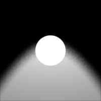
Baked illumination
The baked out point cloud, illumvol.ptc, has around 1.2 million data points:
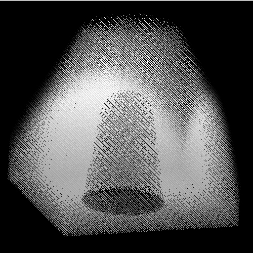
Point cloud of baked illumination values
In these examples, the volume point cloud was baked from a volume shader in PRMan. It is also possible to generate volume point cloud files using other applications than PRMan via the point cloud file API described in Section 8.
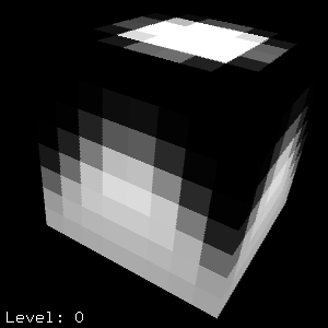
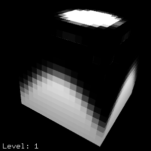
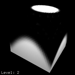
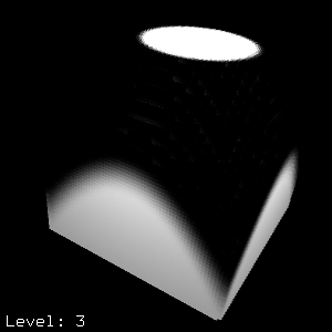
6.3 Creating volume data brick maps
Creating brick maps from volume point clouds is done with brickmake - just as for baked surface data. For example:
brickmake smokevol.ptc smokevol.bkm
brickmake illumvol.ptc illumvol.bkm
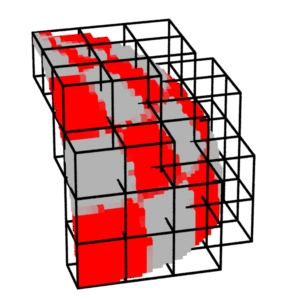
Here is the brick map of the 3D smoke texture:
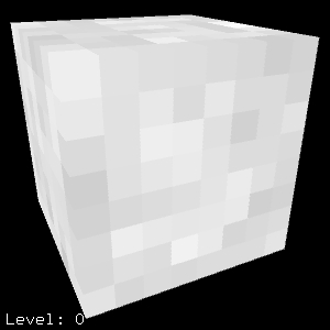
Level 0 |
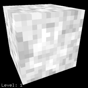
Level 1 |
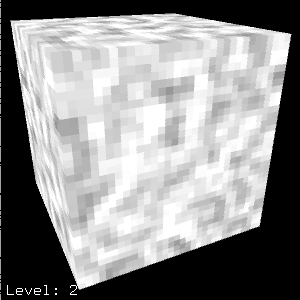
Level 2 |
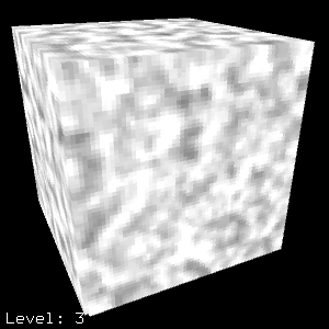
Level 3 |
And here is the brick map of the volume illumination:
Level 0 |
Level 1 |
Level 2 |
Level 3 |
6.4 Example: reading volume data
Now we can render the illuminated smoky volume using ray marching and brick map lookups along the way. Here is the shader:
volume
readillumsmokevol(string illumfilename = "", smokefilename = "";
                  float densitymultiplier = 1;
                  float depth = 1, steps = 100)
{
  color Cv = 0, Ov = 0;   // accumulated color and opacity of volume
  color dCv, dOv;   // differential color and opacity
  color illum;
  point Pfront, Pcurrent;
  normal N0 = 0;
  vector In = normalize(I);
  vector dx = depth/steps * In, offset;
  float smokedensity;
  float ok1, ok2;
  uniform float steplength = depth/steps, step = 0;

  // Compute a start position (jittered in depth)
  Pfront = P - depth * In;
  offset = random() * dx;
  Pcurrent = Pfront + offset;

  // March along a ray through the volume
  while (step < steps) {

    // Lookup the illumination and the smoke density
    ok1 = texture3d(illumfilename, Pcurrent, N0, "illum", illum);
    ok2 = texture3d(smokefilename, Pcurrent, N0, "smokedensity", smokedensity);

    if (ok1 == 1 && ok2 == 1) {
      // Accumulate opacity and scattered illumination
      dOv = densitymultiplier * smokedensity * steplength;
      dCv = illum * dOv;
      Cv += (1-Ov) * dCv;
      Ov += (1-Ov) * dOv;
    }

    // Advance one step
    step += 1;
    Pcurrent += dx;
  }

  Ci = Cv;
  Oi = Ov;
}
Here's the RIB file with the illuminated smoky volume and sphere:
FrameBegin 0

  Format 300 300 1
  シェーディングInterpolation "smooth"
  PixelSamples 4 4
  Display "Reading volume illumination and smoke density" "it" "rgba"
  Quantize "rgba" 255 0 255 0.5
  Projection "orthographic"
  Translate 0 0 10

  WorldBegin

    # Sphere casting a shadow
    AttributeBegin
      # Atmosphere shader ray marches through baked illumination and
      # smoke density in volume
      Atmosphere "readillumsmokevol"
        "illumfilename" "illumvol.bkm" "smokefilename" "smokevol.bkm"
        "depth" 0.7 "steps" 50
      Surface "matte"
      Scale 0.3 0.3 0.3
      Sphere 1 -1 1 360
    AttributeEnd

    AttributeBegin
      # Atmosphere shader ray marches through baked illumination and
      # smoke density in volume
      Atmosphere "readillumsmokevol"
        "illumfilename" "illumvol.bkm" "smokefilename" "smokevol.bkm"
        "depth" 2 "steps" 100
      Surface "constant"
      # Back wall -- necessary to execute the atmosphere shader
      Polygon "P" [-1 -1 1  1 -1 1  1 1 1  -1 1 1]
    AttributeEnd

  WorldEnd
FrameEnd
The rendered image shows the sphere and illuminated smoky volume.
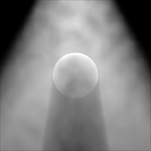
Sphere in illuminated smoky volume
Tip
If volume texture lookups are done at positions outside the volume containing the original data points, the volume lookups will get data values from very coarse levels in the brick map. This can cause blocky artifacts. There are two ways to avoid this:
- Ensure that there are no lookups outside the original volume of the data points.
- Bake additional data points around the original volume. These data should have "neutral" values such as e.g. black color, zero opacity, zero smoke density, etc.
6.5 Discussion
If both density and illumination were baked into the same brick map, only half as many lookups would be necessary, and the run time would be faster.
In the previous example, reading the baked data is not significantly faster than computing the data from scratch. However, some data are more time-consuming to compute, while the lookup time is independent of how long it took to compute the data to begin with.
We have made the simplification that the illumination does not depend on the smoke density between the light source and the illuminated points. If we wanted to compute more accurate illumination, we must ray march through the volume, looking up smoke densities along the way. There are two ways of doing this: the slow way and the fast way.
The slow way: At each point we wish to compute the illumination, we can ray march through the volume between the light source and the point, accumulating smoke densities along the way. This is an order O(n^2) algorithm, with n being the number of points (more than 1 million in this example).
The fast way: It is much more efficient to change the ray marching direction: ray march from the light source through the volume, accumulating the densities along the way and baking the attenuated illumination. This is an order O(n) algorithm - much more manageable.
7 Caching of data
The bake3d() and texture3d() functions have an optional parameter called "cachelifetime". When "cachelifetime" is set, the data points are not written to a point cloud file, but are instead cached in memory. In this case, the "filename" parameter specifies the name of the cache instead of the name of a file. The values of "cachelifetime" can (currently) be "shadinggrid" or "frame".
For "cachelifetime" "shadinggrid", the data are stored in a cache that lives on the shading grid. The cache is cleared when the grid has been shaded. This is mainly useful for sharing common computation results between multiple light source shaders being run to illuminate a surface, for reusing computation results from a displacement shader in a surface shader, and (if filterradius > 0) for sharing results between nearby shading grid points.
For "cachelifetime" "frame", the data are stored in a kd-tree. The kd-tree is cleared when the rendering of a frame is completed. This caching functionality replaces the irradiancecache() "insert" and "query". (Hence the irradiancecache() function has been eliminated.)
The bake3d() and texture3d() cache lifetimes should of course be identical for a given cache name.
We may add other cache lifetimes, for example, "bucket" or "object", in the future.
8 The getpoints() function
NEW FUNCTION in PRMan 16.0: getpoints().
The getpoints function gets data from a specified number of nearest points in point cloud(s). The lookup region is specified by a filterregion for position and one for normals. The lookup routine is the same as for texture3d() lookups in point clouds, but instead of returning a weighted average of the point data, the "raw" point data are returned in arrays of data. If the normal filterregion parameter has normal (0,0,0), it indicates that we don't care about normals, and no points are rejected due to having a normal outside the normal filterregion.
Among many other uses, this function can be used to do isotropic or anisotropic lookups in point clouds, with the shader applying filter weights for anisotropic blur. It can also get e.g. the position of the points in the shading grid that the current shading point is on.
Here is an example of a shader snippet using the getpoints() function:
// Setup filter region for anisotropic point cloud lookups around point P
filterregion frP;
frP->calculate3d(P);
frP->scale(5);
// Setup filter region for normals
normal Nn = normalize(N);
vector T1 = normalize(dPdu);
vector T2 = Nn ^ T1; // T2 = Nn x T1
float conesize = 0.5;
filterregion frN;
frN->calculate3d(Nn, conesize*T1, conesize*T2);
// Read data from point cloud file
npoints = getpoints(filename, frP, frN, maxpoints, "mydata1", md1, "mydata2", md2, ...);
// Loop over data in md array
...
The example above reads data in the channel "mydata1" into the array called md1, and similar for "mydata2". The shader can then e.g. loop over the data in the arrays and compute weighted averages for smooth filtering. This example uses an anisotropic filterregion defined by the viewing angle of the surface at position P. For example, if the surface is seen at a grazing angle at P, then frP will be very elongated, resulting in points relatively close to P being excluded from the filterregion if they are to the side of P, but included if they are in front of or behind P.
For another example, here's a snippet with a getpoints() lookup with isotropic region and normal filterregion (0,0,0):
// Setup filter region for isotropic point cloud lookups around point P
frP->calculate3d(P);
frP->clampaspectratio(1); // make length of shortest axis equal the longest
frP->scale(5);
// Setup dummy filter region for normals
normal N0 = normal(0);
frN->calculate3d(N0, N0, N0);
// Read data from point cloud file
npoints = getpoints(filename, frP, frN, maxpoints, ...);
It is also possible to ask for the special pre-defined data channels "_position", "_normal", and "_radius" even if those have not been explicitly stored in a bake3d() call.
For yet another example, here getpoints() is used to get the data "mydata1" of all points on the shading grid that P is on, sorted according to the distance from P:
// Setup filter region for isotropic point cloud lookups around point P
frP->calculate3d(P);
frP->clampaspectratio(1); // make length of shortest axis equal the longest
frP->scale(100000); // make the filter region huge
// Setup dummy filter region for normals
normal N0 = normal(0);
frN->calculate3d(N0, N0, N0);
// Read data from point cloud file
npoints = getpoints(filename, frP, frN, maxgridpoints, "cachelifetime", "shadinggrid", "sort", 1, "mydata1", md1);
Current limitations for "cachelifetime" "shadinggrid": the order of the data channels has to be the same as in the bake3d() call, and the special pre-defined data channels "_position", "_normal", and "_radius" are not implemented.
9 Common pitfalls and known issues
Be careful about baking at ray hit points! Baking at ray hit points can scatter additional data points in the point cloud, in addition to the regular data baked from REYES shading grids. The additional data points can have widely varying radius values. This is discussed in Section 2.3.
Subsurface scattering and point-based color bleeding from implicit surfaces can be too bright! The points overlap more on implicit surfaces than on other surface types. So any type of computation that relies on the point density, for example subsurface scattering and point-based color bleeding, will be too bright. (Note, however, that area(P, "dicing") and the radius values computed automatically by the bake3d() function are correct on implicit surfaces.)
Don't bake point clouds or brickmake over slow a network! When generating a point cloud or a brick map, write the resulting file to local disk (i.e. the disk associated with the computer doing the work) and then copy the final file across the network. This is faster than writing the file directly to a remote file location because the points and bricks are written in relatively small packets.
10 Frequently asked questions
Q: Why don't you add a loop construct in RenderMan シェーディング Language (SL) that loops over nearby shading points?
A: Only shading points on the same grid would be available during rendering, and this would be of limited use. For example, a shading point on the edge of a shading grid would be missing many of its immediate "neighbor" points.
Q: Why don't you add a loop construct in SL that loops over all nearby points from a point cloud file (baked in a previous pass)?
A: If only points within a specified radius were looped over, this would have limited use: for loops over baked points, one usually wants to not only to loop over the nearby points, but also some coarse representation of more distant points.
Q: Why don't you add a loop construct in SL that loops over both nearby and distant points?
A: For efficiency, the distant points need to be clustered together, otherwise the loops would be extremely slow. The algorithm for computing the coarse clustering representation of distant points depends on the application, so it must be programmable. This is beyond the scope of SL. We believe that for these types of computation, C and C++ are more suitable than SL. Writing a DSO that reads the point cloud (using the point cloud API) and computes a hierarchical representation is much more flexible. The subsurface scattering code in the application note "Translucency and Subsurface Scattering" is an example.
Q: Why are there no API functions for writing data to a brick map?
A: The reason is that this would be hard to do efficiently: if you insert data at one level in the brick map all other levels have to be updated accordingly.
11 More information
The brick map format is a tiled version of the adaptive octree formats used by:
David DeBry, Jonathan Gibbs, Devorah DeLeon Petty, and Nate Robins.
Painting and レンダリング テクスチャs on Unparameterized Models.
SIGGRAPH 2002, pp. 763-768.
David Benson and Joel Davis.
Octree テクスチャs.
SIGGRAPH 2002, pp. 785-790.
The tiling, caching, and filtering aspects are inspired by PRMan's handling of regular 2D textures. This is described in:
Darwyn Peachey.
テクスチャ on Demand.
Pixar Technical Memo 217, 1990.
Global illumination using brick maps is described in:
Per H. Christensen and Dana Batali.
An Irradiance Atlas for Global Illumination in Complex Production Scenes.
レンダリング Techniques '04 (Proceedings of the Eurographics Symposium on レンダリング 2004), pp. 133-141.
PRMan's ambient occlusion and irradiance baking (that also uses point clouds and brick maps) is described in the Ambient Occlusion, Image-Based Illumination, and Global Illumination application note.
The API for reading and writing point clouds is described in The Point Cloud File API. The API for reading brick maps is described in The Brick Map File API.