Point-Based Approximate Ambient Occlusion and カラー Bleeding
Point-Based Approximate Ambient Occlusion and カラー Bleeding
November 2005 (Revised June 2008)
1 Introduction
The purpose of this application note is to provide recipes and examples for computing point-based approximate ambient occlusion and color bleeding using Pixar's RenderMan (PRMan).
The basic idea is to first bake a point cloud containing areas (and optionally color), one point for each micropolygon, to create a point-based representation of the geometry in the scene. Each point is considered a disk that can cause occlusion and/or color bleeding. For efficiency, the algorithm groups distant points (disks) into clusters that are treated as one entity. The computation method is rather similar to efficient n-body simulations in astrophysics and clustering approaches in finite-element global illumination (radiosity). Some of the implementation details also resemble the subsurface scattering method used in PRMan's ptfilter program.
The advantages of our point-based approach are:
- No noise.
- Faster computation times. (No ray tracing.)
- The geometric primitives do not need to be visible for ray tracing; this can significantly reduce the memory consumed during rendering.
- カラー bleeding is nearly as fast as occlusion. (No evaluation of shaders at ray hit points.)
- Computing (HDRI) environment map illumination is just as fast as computing only occlusion.
- Displacement mapped surfaces take no more time than non-displaced surfaces.
- Efficient point and octree caches mean that only a small part of the data need to be kept in memory.
- It runs on standard CPUs - no special hardware required.
The disadvantages are:
- The area (and optionally color) point cloud has to be generated in a pre-pass, making this a two-pass approach.
- The algorithm is not as accurate as ray tracing and should not be used for perfectly specular reflections and refractions.
2 Point-Based Approximate Ambient Occlusion
Computing approximate ambient occlusion requires two steps: 1) generating a point cloud with area data; 2) rendering using the occlusion() function to compute point-based approximate ambient occlusion.
2.1 Baking a Point Cloud with Area Data
First generate a point cloud of area data. Make sure that all objects that should cause occlusion are within the camera view, and add the following attributes to the RIB file:
Attribute "cull" "hidden" 0   # don't cull hidden surfaces
Attribute "cull" "backfacing" 0   # don't cull backfacing surfaces
Attribute "dice" "rasterorient" 0   # view-independent dicing
This will ensure that all surfaces are represented in the point cloud file. Add the following display channel definition:
DisplayChannel "float _area"
And assign this shader to all geometry:
Surface "bake_areas" "filename" "foo_area.ptc" "displaychannels" "_area"
The shader is very simple and looks like this:
surface
bake_areas( uniform string filename = "", displaychannels = "" )
{
  normal Nn = normalize(N);
  float a, opacity;

  a = area(P, "dicing"); // micropolygon area
  opacity = 0.333333 * (Os[0] + Os[1] + Os[2]); // average opacity
  a *= opacity; // reduce area if non-opaque

  if (a > 0)
    bake3d(filename, displaychannels, P, Nn, "interpolate", 1, "_area", a);

  Ci = Cs * Os;
  Oi = Os;
}
レンダリング even complex scenes with this simple shader should take less than a minute. The number of baked points can be adjusted by changing the image resolution and/or the shading rate. It is often sufficient (for good quality in the next step) to render with shading rate 4 or higher. This shader reduces the area of points on semi-transparent surfaces so that they cause less occlusion. (If this behavior is not desired, just comment out the line in which the area is reduced by the opacity.) The opacity could of course come from texture map lookups - instead of being uniform over each surface as in this shader.
As an example, consider the following rib file:
FrameBegin 1
  Format 400 300 1
  PixelSamples 4 4
  シェーディングRate 4
  シェーディングInterpolation "smooth"
  Display "simple_a.tif" "it" "rgba"
  DisplayChannel "float _area"

  Projection "perspective" "fov" 22
  Translate 0 -0.5 8
  Rotate -40  1 0 0
  Rotate -20  0 1 0

  WorldBegin

    Attribute "cull" "hidden" 0   # don't cull hidden surfaces
    Attribute "cull" "backfacing" 0   # don't cull backfacing surfaces
    Attribute "dice" "rasterorient" 0   # view-independent dicing

    Surface "bake_areas" "filename" "simple_areas.ptc"
      "displaychannels" "_area"

    # Ground plane
    AttributeBegin
      Scale 3 3 3
      Polygon "P" [ -1 0 1  1 0 1  1 0 -1  -1 0 -1 ]
    AttributeEnd

    # Sphere
    AttributeBegin
      Translate -0.7 0.5 0
      Sphere 0.5  -0.5 0.5  360
    AttributeEnd

    # Box (with normals facing out)
    AttributeBegin
      Translate 0.3 0 0
      Rotate -30  0 1 0
      Polygon "P" [ 0 0 0  0 0 1  0 1 1  0 1 0 ]   # left side
      Polygon "P" [ 1 1 0  1 1 1  1 0 1  1 0 0 ]   # right side
      Polygon "P" [ 0 1 0  1 1 0  1 0 0  0 0 0 ]   # front side
      Polygon "P" [ 0 0 1  1 0 1  1 1 1  0 1 1 ]   # back side
      Polygon "P" [ 0 1 1  1 1 1  1 1 0  0 1 0 ]   # top
      Polygon "P" [ 0 0 0  1 0 0  1 0 1  0 0 1 ]   # bottom
    AttributeEnd
  WorldEnd
FrameEnd
レンダリング this scene generates a completely uninteresting image but also a point cloud file called 'simple_areas.ptc'. Displaying the point cloud file using the ptviewer program gives the following image:
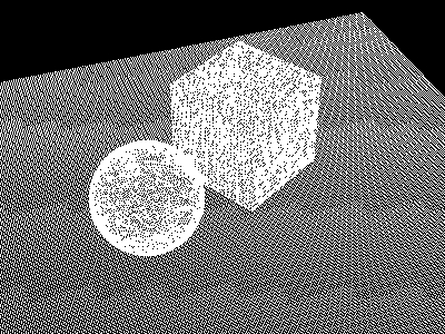
simple_areas.ptc
(Since the areas are tiny, ptviewer will show a black image by default; just select "カラー -> White" to see the points.)
2.2 レンダリング Point-Based Ambient Occlusion
Render the scene with a shader similar to this example:
#include "normals.h"

surface
pointbasedocclusion (string filename = "";
                     string hitsides = "both";
                     float maxdist = 1e15, falloff = 0, falloffmode = 0,
                     samplebase = 0, bias = 0.01,
                     clampocclusion = 1, maxsolidangle = 0.05,
                     maxvariation = 0)
{
  normal Ns = shadingnormal(N);
  float occ;

  occ = occlusion(P, Ns, 0, "pointbased", 1, "filename", filename,
                  "hitsides", hitsides, "maxdist", maxdist,
                  "falloff", falloff, "falloffmode", falloffmode,
                  "samplebase", samplebase, "bias", bias,
                  "clamp", clampocclusion,
                  "maxsolidangle", maxsolidangle,
                  "maxvariation", maxvariation);

  Ci = (1 - occ) * Os;
  Oi = Os;
}
The parameters "hitsides", "maxdist", "falloff", "falloffmode", "samplebase", "bias", and "maxvariation" have the same meaning as for the standard, ray-traced ambient occlusion computation. (Note, however, that using "falloff" 0 with a short "maxdist" gives aliased results. We hope to overcome this limitation in a future release.) There will always be a quadratic falloff due to distance; the "falloff" parameter only specifies additional falloff.
The "samplebase" parameter is a number between 0 and 1 and determines jittering of the computation points. A value of 0 (the default) means no jittering, a value of 1 means jittering over the size of a micropolygon. Setting "samplebase" to 0.5 or even 1 can be necessary to avoid thin lines of too low occlusion where two (perpendular) surfaces intersect.
The "bias" parameter offsets the computation points a bit above the original surface. This can be necessary to avoid self-occlusion on highly curved surfaces and along convex edges. Typical values for "bias" are in the range 0 to 0.01 (depending on the scene size).
The point-based occlusion algorithm will tend to compute too much occlusion. The "clamp" parameter determines whether the algorithm should try to reduce the over-occlusion. Turning on "clamp" roughly doubles the computation time but gives better results. For production-quality rendering, turning on "clamp" is highly recommended.
The "maxsolidangle" parameter is a straightforward time-vs-quality knob. It determines how small a cluster must be (as seen from the point we're computing occlusion for at that time) for it to be a reasonable stand-in for all the points in the cluster. Reasonable values are in the range 0.03 - 0.1.
The "maxvariation" parameter allows interpolation of occlusion across shading grids with low variation in the occlusion values. The default value for maxvariation is 0.0; values such as 0.02 or 0.03 usually give the same image but up to twice as fast. (In PRMan releases prior to 14.0, the "maxvariation" parameter was ignored for point-based calculations.)
Implementation detail: The first time the occlusion() function is executed (with the "pointbased" parameter set to 1) for a given unorganized point cloud file, it reads in the point cloud file and creates an octree. Each octree node has a spherical harmonic representation of the directional variation of the occlusion caused by the points in that node. If the point cloud file is organized, only the file header is read initially and the points and nodes are read on demand and cached - organized point clouds are discussed in further detail below.
RIB file:
FrameBegin 1
  Format 400 300 1
  PixelSamples 4 4
  シェーディングInterpolation "smooth"
  Display "simple_b.tif" "tiff" "rgba"

  Projection "perspective" "fov" 22
  Translate 0 -0.5 8
  Rotate -40  1 0 0
  Rotate -20  0 1 0

  WorldBegin

    Surface "pointbasedocclusion" "filename" "simple_areas.ptc"
      "bias" 0.01 "samplebase" 0.5

    # Ground plane
    AttributeBegin
      Scale 3 3 3
      Polygon "P" [ -1 0 1  1 0 1  1 0 -1  -1 0 -1 ]
    AttributeEnd

    # Sphere
    AttributeBegin
      Translate -0.7 0.5 0
      Sphere 0.5  -0.5 0.5  360
    AttributeEnd

    # Box (with normals facing out)
    AttributeBegin
      Translate 0.3 0 0
      Rotate -30  0 1 0
      Polygon "P" [ 0 0 0  0 0 1  0 1 1  0 1 0 ]   # left side
      Polygon "P" [ 1 1 0  1 1 1  1 0 1  1 0 0 ]   # right side
      Polygon "P" [ 0 1 0  1 1 0  1 0 0  0 0 0 ]   # front side
      Polygon "P" [ 0 0 1  1 0 1  1 1 1  0 1 1 ]   # back side
      Polygon "P" [ 0 1 1  1 1 1  1 1 0  0 1 0 ]   # top
      Polygon "P" [ 0 0 0  1 0 0  1 0 1  0 0 1 ]   # bottom
    AttributeEnd
  WorldEnd
FrameEnd
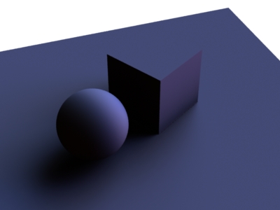
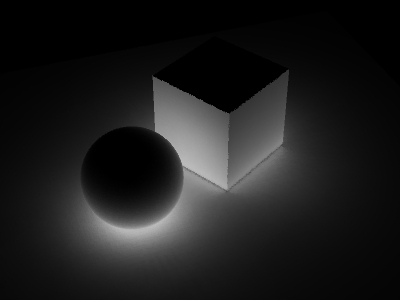
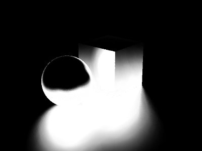
Running this RIB file results in the following image:
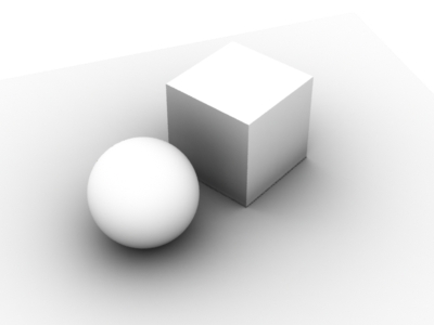
Simple scene with point-based approximate occlusion
The point-based ambient occlusion computation is typically 5-8 times faster than ambient occlusion using ray tracing - at least for complex scenes. (However, if the scene consists only of a few undisplaced spheres and large polygons, as in this example, ray tracing is faster since ray tracing those geometric primitives does not require fine tessellation.)
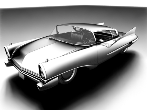
Here is an example of point-based ambient occlusion in a more complex scene:
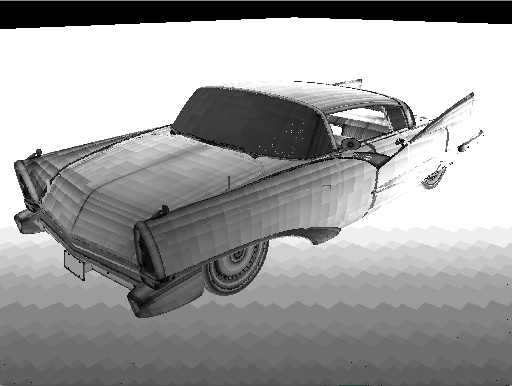
Area point cloud for car (8.2 million points) |
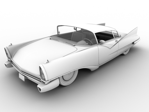
Car with point-based approximate occlusion |
Generating the area point cloud takes about ten seconds on a standard multi-core PC, and computing (and rendering) the point-based ambient occlusion takes about one minute.
2.3 Fine Tuning
Keep in mind that the point-based ambient occlusion values are (by their very nature) not exactly the same as the ambient occlusion computed by ray tracing. However, the point-based occlusion has much of the same "look". It is often necessary to try different combinations of "hitsides", "maxdist", "falloff", "falloffmode", "clamp", and "maxsolidangle" to get an occlusion result that closely resembles ray-traced ambient occlusion. For high-quality results we recommend "hitsides" "both", "clamp" 1, and "maxsolidangle" at most 0.05. Experiment with different settings for bias - typically values in the range 0.0001 to 0.01 are good (depending on the scene size).
Another issue that can require some fine-tuning can occur where two surfaces intersect. Sometimes a thin line with too little occlusion can be visible along the intersection. To avoid this, set the "samplebase" parameter to around 0.01, "hitsides" to "both", and "clamp" to 1, and experiment with different values for the "bias" parameter.
2.4 Environment Directions
The environment direction (the average unoccluded direction, also known as "bent normal") can also be computed by the occlusion() function with the point-based approach. Just pass the occlusion() function an "environmentdir" variable, and it will be filled in - just as for ray-traced occlusion() calls. The environment directions will be computed more accurately if the "clamp" parameter is set than if it isn't.
2.5 Environment Illumination
Environment illumination, as for example from an HDRI environment map, can be computed efficiently as a by-product of the point-based occlusion computation.
For an example, replace the surface shader in the example above with:
#include "normals.h"

surface
pointbasedenvcolor (string filename = "";
                    string hitsides = "both";
                    float maxdist = 1e15, falloff = 0, falloffmode = 0;
                    float samplebase = 0, bias = 0.01;
                    float clampocclusion = 1;
                    float maxsolidangle = 0.05, maxvariation = 0;
                    string envmap = "" )
{
    normal Ns = shadingnormal(N);
    color envcol = 0;
    vector envdir = 0;
    float occ;

    occ = occlusion(P, Ns, 0, "pointbased", 1, "filename", filename,
                    "hitsides", hitsides,
                    "maxdist", maxdist, "falloff", falloff,
                    "falloffmode", falloffmode,
                    "samplebase", samplebase, "bias", bias,
                    "clamp", clampocclusion,
                    "maxsolidangle", maxsolidangle,
                    "maxvariation", maxvariation,
                    "environmentmap", envmap,
                    "environmentcolor", envcol,
                    "environmentdir", envdir
                   );

    Ci = envcol;
    Oi = Os;
}
Change the surface shader call in the rib file to:
Surface "pointbasedenvcolor" "filename" "simple_areas.ptc"
  "envmap" "rosette_hdr.tex"
  "samplebase" 0.001
The resulting image looks like this:
Simple scene with point-based environment illumination
The environment colors are computed much more accurately if the "clamp" parameter is set than if it isn't. Either way, computing point-based environment illumination takes nearly no extra time when point-based occlusion is being computed.
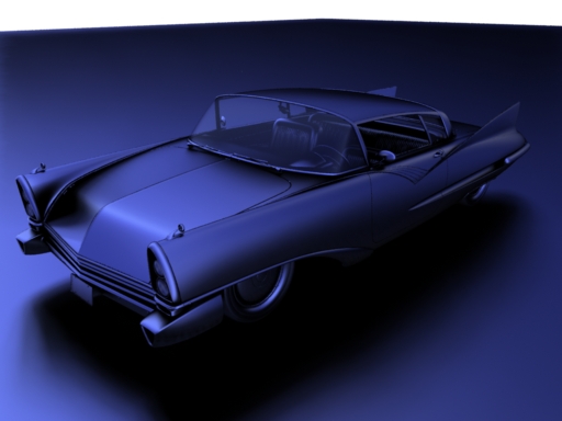
Here's another example of environment illumination, this time the scene is slightly more complex and the environment map consists of two very bright area lights, one green and one blue:
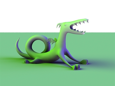
Dragon with point-based environment illumination
2.6 Reflection Occlusion
Reflection occlusion is a popular way to figure out where the reflections are in a scene. At the points with no reflection it is common to look up in a reflection map or environment map. Reflection occlusion is usually computed by tracing rays in a (narrow) cone around the main reflection direction. However, it is also possible to compute reflection occlusion with point-based techniques - as long as the cone is not too narrow.
Here is an example of a shader that computes point-based reflection occlusion:
surface
pointbasedreflectionocclusion (string filename = "";
                 string hitsides = "both";
                 string distribution = "cosine";
                 float clamp = 1;
                 float maxdist = 1e15, falloff = 0, falloffmode = 0;
                 float coneangle = 0.2;
                 float maxsolidangle = 0.01;
                 float samplebase = 0.0;
                 float bias = 0.0001; )
{
    normal Nn = normalize(N);
    vector refl = reflect(I, Nn);
    float occ;

    occ = occlusion(P, refl, 0, "pointbased", 1, "filename", filename,
                    "hitsides", hitsides, "distribution", distribution,
                    "clamp", clamp,
                    "maxdist", maxdist, "falloff", falloff,
                    "falloffmode", falloffmode,
                    "coneangle", coneangle,
                    "maxsolidangle", maxsolidangle,
                    "samplebase", samplebase, "bias", bias);

    Ci = 1 - occ;
    Ci *= Os;
    Oi = Os;
}
As an example, consider again the simple scene with a sphere and a cube on a ground plane. The point cloud and rib files are the same as in the simple example in section 2.2 (above) except that the cube has been moved up a bit higher from the ground plane and the shader is changed to:
Surface "pointbasedreflectionocclusion" "filename" "reflocc_areas.ptc"
    "coneangle" 0.4 "maxsolidangle" 0.005
To get sufficiently accurate reflection occlusion results, the maxsolidangle parameter has to be set to very low values. In this example, we have used a maxsolidangle value of 0.005. (In PRMan 15.0 and higher, we also recommend increasing the rasterresolution parameter from its default value of 12 to 20 or even 30.) The images below show two examples with coneangle 0.4 and 0.2 radians, respectively.
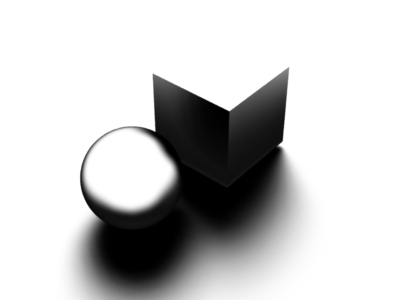
Coneangle 0.4 radians |
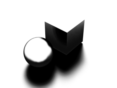
Coneangle 0.2 radians |
Here is an example for more complex geometry. The figure on the left below shows a car with pure point-based reflection occlusion (coneangle 0.3). On the right, the reflection occlusion is enhanced by environment map lookups in the unoccluded directions -- done by passing an "environmentmap" parameter to the occlusion() function and using the resulting "environmentcolor" value. Most of the reflections are blue as the majority of the sky, but some reflection directions are facing more toward clouds and hence those reflections are whiter.
Car with point-based reflection occlusion |
Car with additional environment reflection (sky texture) |
Generally speaking, computing narrow reflection occlusion using the point-based occlusion approach is pushing the algorithm to the limits of what it was designed for. For very narrow cone angles, ray tracing remains the best method to compute reflection occlusion. As a rule of thumb, point-based reflection occlusion works best if the coneangle is at least 0.2 radians, and the occluding objects are not right next to the points where the occlusion is being computed.
3 Point-Based Approximate カラー Bleeding
Computing approximate color bleeding is done in two steps: 1) generating a point cloud with area and color data; 2) rendering using the indirectdiffuse() function to compute point-based approximate color bleeding.
3.1 Baking a Point Cloud with Area and Radiosity Data
The first color bleeding step is similar to the first occlusion step, but also bakes radiosity values. The radiosity values represent diffusely reflected direct illumination, and can be computed, for example, like this:
surface
bake_radiosity(string bakefile = "", displaychannels = "", texturename = "";
               float Ka = 1, Kd = 1)
{
  color irrad, tex = 1, diffcolor;
  normal Nn = normalize(N);
  float a = area(P, "dicing"); // micropolygon area (is 0 on e.g. curves)

  // Compute direct illumination (ambient and diffuse)
  irrad = Ka*ambient() + Kd*diffuse(Nn);

  // Lookup diffuse texture (if any)
  if (texturename != "")
    tex = texture(texturename);

  diffcolor = Cs * tex;

  // Compute Ci and Oi
  Ci = irrad * diffcolor * Os;
  Oi = Os;

  if (a > 0) {
    // Store area and Ci in point cloud file
    bake3d(bakefile, displaychannels, P, Nn, "interpolate", 1,
           "_area", a, "_radiosity", Ci, "Cs", diffcolor);
  }
}
(Here we also bake out the diffuse surface color. That color isn't used in this example, but can be be used to compute multiple bounces of color bleeding using ptfilter, as discussed below.)
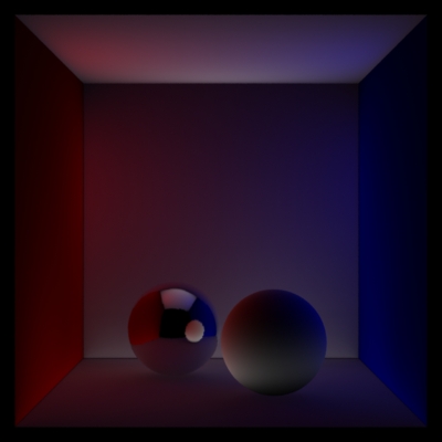
Here is a RIB file showing an example. This scene is the infamous Cornell box with two spheres.
FrameBegin 1
  Format 400 400 1
  シェーディングInterpolation "smooth"
  PixelSamples 4 4
  Display "cornell_a.tif" "it" "rgba"
  Projection "perspective" "fov" 30
  Translate 0 0 5

  DisplayChannel "float _area"
  DisplayChannel "color _radiosity"
  DisplayChannel "color Cs"

  WorldBegin

    Attribute "cull" "hidden" 0   # to ensure occl. is comp. behind objects
    Attribute "cull" "backfacing" 0 # to ensure occl. is comp. on backsides
    Attribute "dice" "rasterorient" 0   # view-independent dicing

    LightSource "cosinelight_rts" 1 "from" [0 1.0001 0] "intensity" 4

    Surface "bake_radiosity" "bakefile" "cornell_radio.ptc"
      "displaychannels" "_area,_radiosity,Cs" "Kd" 0.8

    # Matte box
    AttributeBegin
      カラー [1 0 0]
      Polygon "P" [ -1 1 -1  -1 1 1  -1 -1 1  -1 -1 -1 ]   # left wall
      カラー [0 0 1]
      Polygon "P" [ 1 -1 -1  1 -1 1  1 1 1  1 1 -1 ]   # right wall
      カラー [1 1 1]
      Polygon "P" [ -1 1 1  1 1 1  1 -1 1  -1 -1 1 ]   # back wall
      Polygon "P" [ -1 1 -1  1 1 -1  1 1 1  -1 1 1 ]   # ceiling
      Polygon "P" [ -1 -1 1  1 -1 1  1 -1 -1  -1 -1 -1 ]   # floor
    AttributeEnd

    Attribute "visibility" "transmission" "opaque" # the spheres cast shadows

    # Left sphere (chrome; set to black in this pass)
    AttributeBegin
      color [0 0 0]
      Translate -0.3 -0.69 0.3
      Sphere 0.3  -0.3 0.3  360
    AttributeEnd

    # Right sphere (matte)
    AttributeBegin
      Translate 0.3 -0.69 -0.3
      Sphere 0.3  -0.3 0.3  360
    AttributeEnd
  WorldEnd
FrameEnd
Running this RIB file results in the following image:

Cornell box with spheres
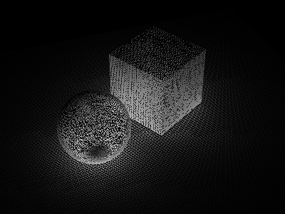
The generated point cloud, cornell_radio.ptc, contains approximately 545,000 points. The figure below shows two views of it (with the radiosity color shown):
cornell_radio.ptc (full view) |
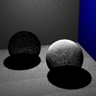
cornell_radio.ptc (partial view) |
3.2 レンダリング Point-Based カラー Bleeding
Now we are ready to compute and render point-based color bleeding using the indirectdiffuse() function. This can be done using a shader similar to this example:
#include "normals.h"

surface
pointbasedcolorbleeding (string filename = "", sides = "front";
                         float clampbleeding = 1, sortbleeding = 1,
                         maxdist = 1e15, falloff = 0, falloffmode = 0,
                         samplebase = 0, bias = 0,
                         maxsolidangle = 0.05, maxvariation = 0;)
{
  normal Ns = shadingnormal(N);
  color irr = 0;
  float occ = 0;

  irr = indirectdiffuse(P, Ns, 0, "pointbased", 1, "filename", filename,
                        "hitsides", sides,
                        "clamp", clampbleeding,
                        "sortbleeding", sortbleeding,
                        "maxdist", maxdist, "falloff", falloff,
                        "falloffmode", falloffmode,
                        "samplebase", samplebase, "bias", bias,
                        "maxsolidangle", maxsolidangle,
                        "maxvariation", maxvariation);

  Ci = Os * Cs * irr;
  Oi = Os;
}
The indirectdiffuse() function has a parameter called sortbleeding. (Clamp must be 1 for it to have any effect.) When sortbleeding is 1, the bleeding colors are sorted according to distance and composited correctly, i.e. nearby points block light from more distant points. This gives more correct colors and deeper (darker) shadows. When sortbleeding is 0, colors from each direction are mixed with no regard to their distance. 0 is the default.
For the rendering pass, the Cornell Box RIB file looks like this:
FrameBegin 1
  Format 400 400 1
  シェーディングInterpolation "smooth"
  PixelSamples 4 4
  Display "cornell_b.tif" "it" "rgba"
  Projection "perspective" "fov" 30
  Translate 0 0 5

  WorldBegin

    Attribute "visibility" "specular" 1 # make objects visible to refl. rays
    Attribute "trace" "bias" 0.0001

    Surface "pointbasedcolorbleeding" "filename" "cornell_radio.ptc"
      "clampbleeding" 1 "sortbleeding" 1 "maxsolidangle" 0.03
      "maxvariation" 0.02

    # Matte box
    AttributeBegin
      カラー [1 0 0]
      Polygon "P" [ -1 1 -1  -1 1 1  -1 -1 1  -1 -1 -1 ]   # left wall
      カラー [0 0 1]
      Polygon "P" [ 1 -1 -1  1 -1 1  1 1 1  1 1 -1 ]   # right wall
      カラー [1 1 1]
      Polygon "P" [ -1 1 1  1 1 1  1 -1 1  -1 -1 1 ]   # back wall
      Polygon "P" [ -1 1 -1  1 1 -1  1 1 1  -1 1 1 ]   # ceiling
      Polygon "P" [ -1 -1 1  1 -1 1  1 -1 -1  -1 -1 -1 ]   # floor
    AttributeEnd

    Attribute "visibility" "transmission" "opaque" # the spheres cast shadows

    # Left sphere (chrome)
    AttributeBegin
      Surface "mirror"
      Translate -0.3 -0.69 0.3
      Sphere 0.3  -0.3 0.3  360
    AttributeEnd

    # Right sphere (matte)
    AttributeBegin
      Translate 0.3 -0.69 -0.3
      Sphere 0.3  -0.3 0.3  360
    AttributeEnd
  WorldEnd
FrameEnd
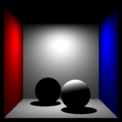
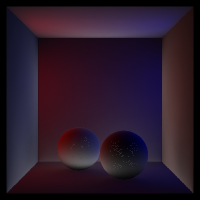
Here are two versions of the rendered image showing color bleeding:
Cornell box color bleeding (sortbleeding 0) |
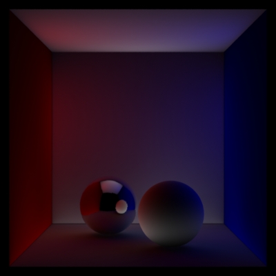
Cornell box color bleeding (sortbleeding 1) |
The shadows under the sphere are much darker in the image to the right due to "sortbleeding" being 1.
This example only shows the indirect illumination. If the shader also computes the direct illumination, a full global illumination image can be rendered.
If the indirectdiffuse() function is passed a parameter called "occlusion" it will also compute point-based approximate ambient occlusion and assign it to that parameter. If the indirectdiffuse() function is passed a parameter called "environmentdir" it will compute an environment direction (average unoccluded direction, also known as "bent normal").
The computation of color bleeding can be combined with environment map illumination - just as for occlusion. Simply pass an "environmentmap" parameter to the indirectdiffuse() function.
It is important to note that there is very little run-time increase from computing occlusion to computing color bleeding. This is in contrast to ray tracing, where the cost of evaluating shaders at the ray hit points is often considerable.
The parameter "areachannel" can be used to specify the name of the channel (in the input point cloud) that contains area data. The default channel name is "_area". Similarly, the parameter "radiositychannel" can be used to specify the name of the channel with radiosity data. The default channel name is "_radiosity".
In PRMan 15.2 the "hitsides" parameter was split into two for finer control: "colorhitsides" and "occlusionhitsides". The default for both is "both". Best results are obtained with "colorhitsides" "front" and "occlusionhitsides" "both". For backwards compatibility, the "hitsides" parameter sets both (and is also used for ray tracing).
3.3 A More Complex Example
Here is an example of point-based color bleeding in a more complex scene:
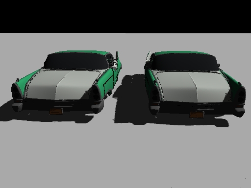
Radiosity point cloud for two cars (9 million points) |
Cars with point-based color bleeding |
Generating this radiosity point cloud takes about three minutes on a standard PC, and computing (and rendering) the point-based color bleeding takes around 9 minutes. Notice the strong green color bleeding from the cars, and the gray color bleeding from the ground onto the cars.
It is worth pointing out that the objects can have textures and displacement shaders without increasing the run-time for baking and rendering.
3.4 Glossy Reflections
Point-based computations can also be used to compute approximate glossy reflections. This is done by passing the indirectdiffuse() function a reflection direction and a fairly narrow cone.
surface
pointbasedglossyreflection (string filename = "", sides = "front";
                            float clampbleeding = 1, sortbleeding = 1,
                            maxdist = 1e15, falloff = 0, falloffmode = 0,
                            coneangle = 0.2,
                            samplebase = 0.0, bias = 0.01,
                            maxsolidangle = 0.01;)
{
  normal Nn = normalize(N);
  vector refl = reflect(I, Nn);
  color irr;

  irr = indirectdiffuse(P, refl, 0, "pointbased", 1, "filename", filename,
                        "hitsides", sides, "clamp", clampbleeding,
                        "sortbleeding", sortbleeding,
                        "maxdist", maxdist, "falloff", falloff,
                        "falloffmode", falloffmode,
                        "coneangle", coneangle,
                        "samplebase", samplebase, "bias", bias,
                        "maxsolidangle", maxsolidangle);

  Ci = Os * Cs * irr;
  Oi = Os;
}
Computing glossy reflections this way is (nearly) as fast as reflection occlusion. Below is an example showing baking (left) and glossy reflection of the baked point cloud (right).
Baked radiosity values (700,000 points) |
Glossy reflections |
Just as for the color bleeding case, the indirectdiffuse() can be passed an environment map parameter for glossy reflection calculations. The environment map colors will contribute color in directions with no baked points.
Of course, since the reflected colors are baked, they may not have highlights in the right places. But the glossy reflections are so blurry that that oftentimes doesn't matter.
Just as for reflection occlusion, point-based glossy reflections work best if the coneangle is at least 0.2 radians and the maxsolidangle value is small. We also recommend (in PRMan 15.0 and higher) to use a higher rasterresolution than the default 12.
4 Point-Based Area Light Sources
Illumination from area light sources can be computed as a special case of color bleeding.
4.1 Baking Area Light Sources and Shadow Casters
The first step is to bake a point cloud with colored points from the light source objects, and black points from the shadow caster objects. The light sources and shadow casters can be any type of geometry, which makes this approach very flexible - the geometry can even be displacement-mapped. The light source intensity can be constant or computed procedurally or using a texture.
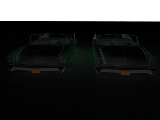
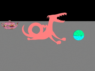
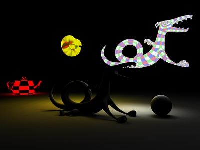
The following example shows three area light sources: a teapot, a sphere, and a dragon. The area lights illuminate a scene with three objects: a dragon, a sphere, and a ground plane.
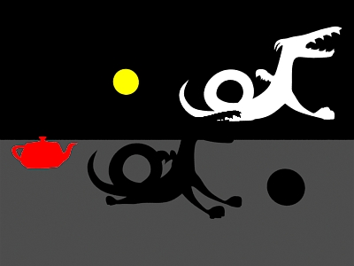
Area light sources and shadow casters
The result of this rendering is a point cloud containing very bright points from the light sources and black points from the shadow-casting objects. (For this scene, no points were baked from the ground plane since it is neither supposed to emit light nor cast shadows.)
4.2 Computing Illumination
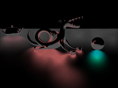
For this step, the same shader (pointbasedcolorbleeding) as above is used. it is important to set (keep) the "clamp" and "sortbleeding" parameters to 1. The image below shows color bleeding computed from the area light source point cloud:
Dragon, sphere, and plane with area lights and soft shadows
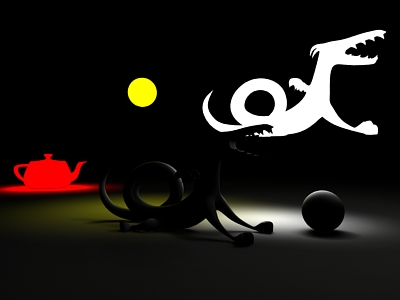
Below is another variation of this scene. Here the teapot light source has a procedural checkerboard texture, the sphere light source is displacement-mapped and texture-mapped, and the dragon light source is texture-mapped as well. (In this image, the light source objects are rendered dimmer than the colors used for baking their emission - this is to avoid over-saturation that makes the textures hard to see.)
テクスチャd and displaced area light sources
5 Point-Based Computations using ptfilter
Instead of rendering the occlusion and/or color bleeding, it can be useful to compute the data as a point cloud. This makes later reuse simple, and also makes it possible to generate a brick map (which has better caching properties than point clouds) of the data.
5.1 Occlusion
Given one or more point clouds with area data, we can run the ptfilter program. The syntax is:
ptfilter -filter occlusion [options] areafiles occlusionfile
The last filename is the name of the resulting occlusion point cloud file; all preceeding filenames are the names of the (source) area point cloud files. For example:
ptfilter -filter occlusion -maxsolidangle 0.05 foo_areas.ptc foo_occl.ptc
This generates a point cloud with occlusion data. Optional parameters for ptfilter in occlusion mode are:
maxsolidangle (float) determines the accuracy of the computation (measured in radians, default is 1 which gives very rough results);
rasterresolution (int) determines the resolution of the pixel raster used when clamp is on (the default is 12);
samplebase (float) jitters the computation over a small disk around the computation point (value should be between 0 and 1, default is 0);
bias (float) offset of computation point in normal direction (measured in scene units, default is 0);
- sides [front|back|both] determines which sides should contribute
occlusion (default is both);
clamp [0|1] determines whether over-occlusion should be reduced (default is 1);
envdirs [0|1] compute environment directions (average unoccluded directions aka. "bent normals", default is 0);
maxdist f, -falloff f, and -falloffmode [0|1] determine the occlusion falloff with distance (defaults are 1e15, 0.0, and 0, respectively);
distribution [cosine|uniform] determines the distribution (weighting) of occlusion over the hemisphere (default is cosine);
coneangle (float) specifies the hemisphere fraction that contributes occlusion (a value in radians between 0 and pi/2, default is pi/2, values below 0.2 are not recommended);
sources (filenames) can be used if there is more than one point cloud with area data - see below;
positions (filenames) can be used if the computation points differ from the point positions in the area point cloud(s) - see below;
output (filename) is the name of the output file (necessary if there are source and/or position point clouds specified) -- see below;
progress [0|1|2] print progress reports during computation (default is 0);
newer [0|1] only recompute if the input point cloud(s) are newer than the output point cloud (default is 0);
thread (int) the number of threads to use for the computation (default is 1);
areachannel (string) is the name of the channel (in the input point cloud) with area data (default is "_area");
reflectiondirchannel (string) is the optional name of a channel containing reflection directions - used to compute reflection occlusion (default is "").
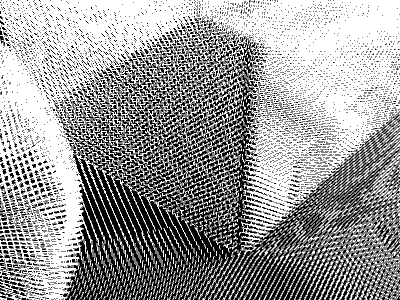
The computed occlusion point cloud for the simple scene looks like this:
Point cloud with ambient occlusion values |
Point cloud with ambient occlusion values (shown as facets) |
The point cloud can now be used to generate a brick map of the occlusion values, if desired:
brickmake simple_occl.ptc simple_occl.bkm
As mentioned above, set the optional -envdirs parameter to 1 if the environment directions should be computed in addition to the occlusion. For example:
ptfilter -filter occlusion -maxsolidangle 0.05 -envdirs 1 foo_areas.ptc foo_occl.ptc
Here are the computed environment directions in the resulting point cloud:
Point cloud with environment directions (zoomed in)
ptfilter can also compute reflection occlusion. This requires that the point cloud has baked-in reflection directions (in addition to the areas). If the reflection directions have been baked in a vector called e.g. _refldir, ptfilter can be called like this:
ptfilter -filter occlusion -clamp 1 -coneangle 0.2 -maxsolidangle 0.01 -reflectiondirchannel _refldir foo_refldirs.ptc foo_refloccl.optc
Here is an image showing an example of reflection occlusion:
Point cloud with reflection occlusion values (shown as facets)
ptfilter cannot currenly compute environment illumination.
For added flexibility, it is also possible to separately specify the positions where occlusion should be computed. The positions are given by points in a separate set of point cloud files. The syntax is as follows:
ptfilter -filter occlusion [options] -sources filenames -positions filenames -output filename
For example:
ptfilter -filter occlusion -maxsolidangle 0.1 -sources foo_areas.ptc -positions foo_pos.ptc -output foo_occl.ptc
In this example there is only one file with areas and one file with positions; but each set of points can be specified by several point cloud files. If no position files are given, the point positions in the area point clouds are used.
5.2 カラー Bleeding
Similar to the point-based occlusion computation, ptfilter can also compute color bleeding. This is done as follows:
ptfilter -filter colorbleeding -maxsolidangle 0.05 -sides front foo_radio.ptc foo_bleed.ptc
Here are two different views of the color bleeding point cloud for the Cornell box scene:
Cornell box color bleeding point cloud (full view) |
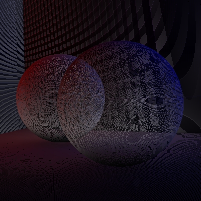
Cornell box color bleeding point cloud (partial view) |
In addition to the optional parameters for occlusion mode, there are a few optional parameters specifically for colorbleeding mode:
- sortbleeding [0|1] reduces mixing of near-vs-far colors by sorting the color contributions and compositing them near over far (default is 0);
- bounces (int) specifies the number of bounces of color bleeding (default is 1) - for this to work, the original point cloud file must contain Cs data in addition to the area and radiosity data;
- radiositychannel (string) is the name of the channel (in the input point cloud) with radiosity data. The default channel name is "_radiosity".
- colorsides [front|back|both] and occlusionsides [front|back|both] These are similar to the "colorhitsides" and "occlusionhitsides" parameters to indirectdiffuse().
The parameter -clamp reduces over-bleeding - just like it reduces over-occlusion.
As for occlusion computations, there can be a separate set of point clouds specifying where to compute the colorbleeding.
The data in the computed point cloud file are called "_occlusion" and "_indirectdiffuse" and optionally "_environmentdir".
5.3 Area ライト
ptfilter can also compute soft illumination and shadows from area light sources. Simply bake a point cloud with brightly colored points at the area lights and black points at the shadow casters. Then run ptfilter -filter colorbleeding as in the previous section. Remember to set -clamp 1 and -sortbleeding 1 for best results.
6 Using Organized Point Clouds
A limitation of standard point clouds is that the entire point cloud has to be read in by texture3d() and all the points stay in memory. In order to handle large point clouds more efficiently, PRMan 14.0 introduced a new file format: organized point cloud. An organized point cloud is a collection of points organized into an octree. The octree nodes can have additional data associated with them or not (depending on the application). For organized point clouds, texture3d() reads the points and octree nodes on demand, and cache them in a fixed-size cache.
Creating Organized Point Clouds</h3>
As described in the Baking 3D テクスチャs application note, ptfilter -filter organize is used to generate an organized point cloud for use with texture3d().
In addition, ptfilter with the ssdiffusion, occlusion, and colorbleeding filters also generates organized point clouds by default. (There is one exception: if a point cloud of compute positions is specified the output will be written "on-the-fly" into an unorganized point cloud with the points in the same order as in the point cloud that specified the compute positions.)
To determine whether a point cloud file is organized or not, just run ptviewer -info foo.ptc or ptviewer -onlyinfo foo.ptc. The point cloud is organized if the listed number of tree nodes is larger than zero.
6.1 Partial Evaluation
Organized point clouds can also be used to render subsurface scattering, ambient occlusion, and color bleeding more efficiently. This is done by letting ptfilter do a partial evaluation of the data, write the partial evaluation results as an organized point cloud, and then calling subsurface(), occlusion(), or indirectdiffuse() during rendering. For example, to generate an organized point cloud for use with the point-based indirectdiffuse() function, the following command is used:
ptfilter -filter colorbleeding -partial 1 -sides front foo_radio.ptc foo_radio.optc
The points in the organized point cloud contain the same data as the input point cloud but are sorted. In addition, each octree node contains a bounding box of the points in the octree node, as well as additional data. (For color bleeding, the additional data are the centroid and total area of the points in the node and spherical harmonics representing the directional variation of the emitted power and projected area of the points in the node.) This information is used by the subsurface(), occlusion(), and indirectdiffuse() functions during rendering. In fact, when this information has not been precomputed, computing it is the first thing these functions have to do.
When precomputing the partial information for occlusion and color bleeding, it is important that the -sides parameter (front, back, or both) corresponds to the intended use in the shading functions (usually both for occlusion and front for color bleeding). All other parameters are ignored during partial evaluations.
-partial 1 can be combined with -bounces values greater than 1. In this case, ptfilter will compute b-1 bounces and set up the points and octree nodes such that the indirectdiffuse() function can compute the last bounce efficiently.
6.2 Caches
The texture3d(), subsurface(), point-based occlusion(), and indirectdiffuse() functions read groups of points and octree nodes from organized point clouds on demand and cache them. These functions use much less memory when reading organized point cloud files than when reading unorganized point cloud files. (If the functions are given an old-fashioned unorganized point cloud, they revert to the old behavior: the entire point cloud is read in and an octree is built in memory.)
Cache statistics can be found in XML stats files under the heading point/octreeCache. The default cache sizes are 10MB (but no memory is allocated if the caches are not used). How to adjust the cache sizes is described in the cache sizes section of the Baking 3D テクスチャs application note.
7 Miscellanea
7.1 Known Limitations
The current implementation can give discontinuous, aliased results if "falloff" is set to 0 and "maxdist" is shorter than the scene extent. (The default for "maxdist" is 1e15.) With short "maxdist" values, please use falloff 1 or 2. If you must use "falloff" 0, setting "maxsolidangle" to a very small value can reduce the aliasing (but also increases render time significantly).
7.2 Debugging
If the computed occlusion or color bleeding is incorrect in a region of the scene, a good debugging method is to inspect the (area or radiosity) point cloud in that region using ptfilter in the disk or facet display mode. Is the disk representation of the surface a reasonable approximation of the original surface? If not, the shading rate for baking that object may need to be reduced in order to generate more, smaller disks that represent the surface better. If the area/radiosity point cloud is not a decent approximation of the surfaces, the point-based method cannot compute good results.
7.3 Discussion
Some scenes are simply too complex to be ray-traced - storing all the geometry uses more memory than what is available on the computer. For such scenes, point-based occlusion may be the only viable way to compute occlusion. As mentioned earlier, the area point clouds can be sparser than the accuracy of the final rendering, so even ridiculously complex scenes can be handled.
Another use of point-based occlusion is in a workflow that computes occlusion for each frame. Each frame is first rendered coarsely to generate a rather sparse area point cloud. Then the frame is rendered with occlusion using the occlusion() function (with "pointbased" 1) at final resolution. The resulting image can be used as a 2D occlusion layer for compositing, and the point cloud can be deleted. Note that this workflow does not involve any point clouds or brick maps that have to be kept in the file system; the only result that is kept for later compositing is the full-frame occlusion-layer image.
7.4 More Information
More information about the algorithms used for the point-based computations can be found in the following book chapter and technical memo:
- Per H. Christensen. "Point Clouds and Brick Maps for Movie Production". Chapter 8.4 in Markus Gross and Hanspeter Pfister, editors, Point-Based Graphics. May 2007.
- Per H. Christensen. "Point-Based Approximate カラー Bleeding". Pixar Technical Memo #08-01. July 2008.