Improved Subsurface Scattering
Improved Subsurface Scattering
January 2013
1 Introduction
Subsurface scattering is responsible for effects like color bleeding inside materials and the diffusion of light across shadow boundaries. Subsurface scattering is an important effect for realistic rendering of translucent materials such as skin, flesh, fat, fruits, milk, wax, and marble. Previously, PRMan has used the popular dipole diffusion model [Jensen01], [Jensen02] for subsurface scattering. However, the dipole diffusion model is overly smooth, and produces subsurface scattering which looks a lot like wax - which is fine if you're rendering a candle but not ideal if you're trying to render e.g. human skin.
In this application note we will describe the use of a new model for subsurface scattering. The new model produces results that look similar to quantized diffusion [dEon11] but it is faster to evaluate and more numerically stable. The new model was developed in collaboration with Ralf Habel and Wojciech Jarosz at Disney Research Zurich; technical details can be found in the paper listed below [Habel13]. The model divides the subsurface scattering into an accurate single-scattering term and a diffusion term that represents multi-scattering.
The new subsurface scattering model is called beam diffusion and is introduced in PRMan version 18.0. It is fully compatible with the previous dipole model, meaning that the ptfilter program and the subsurface() function use the new model with the same parameters as for the dipole diffusion model. As before, the subsurface function can use ray tracing or point clouds. Although the new model is more accurate, there is only a modest increase in render time.
2 Motivation: a reference solution
The following image shows a reference image of subsurface scattering computed using a brute-force Monte Carlo path tracer:
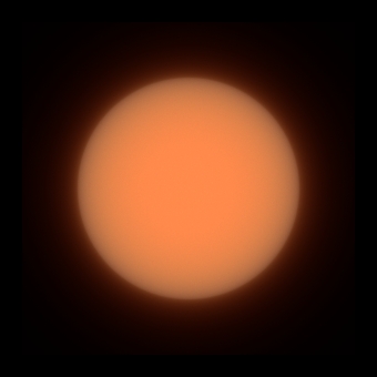
Reference image of subsurface scattering on skin
This look is what we're aiming for when rendering subsurface scattering - but it is much too slow to compute this way, so we use faster approximations as described in the following sections.
In the approximations, we often separate out single-scattering from multiple scattering. To make this distinction clearer, we show this separation also for the MC reference image: the top third of the image shows single scattering, the middle third shows multiple scattering (up to hundreds of bounces), and the bottom third shows all scattering (single plus multiple). The scattering parameters are for the skin1 material from [Jensen01]: reduced extinction coefficients = sigma'_s = (0.74 0.88 1.01), absorption = sigma_a = (0.032 0.17 0.48), index of refraction = ior = 1.3. 10 billion particles were emitted to generate this image; tracing them takes several hours of computation time even for this very simple scene (a square illuminated by a disk light source).
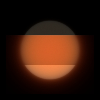
Reference image of subsurface scattering: single scattering, multi scattering, all (single+multi) scattering
3 Subsurface scattering approximations
The image below shows six different approximations of the reference solution discussed above. The left column shows the old approximations, and the right column the new ones (available in PRMan 18.0 and higher).
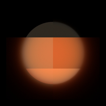
Various types of subsurface scattering
The top row shows two representations of single scattering. On the left is a matte material with ideal diffuse reflection (a brdf: pure surface reflection, no subsurface scattering). On the right is the new single-scattering term; it is an exact match of the Monte Carlo single-scattering reference.
The middle row shows two diffusion approximations of multiple scattering. On the left is the classic dipole diffusion model. It is too smooth and has the wrong hue (and is even too bright overall - here the Ksss value was dialed down to 0.82 to match the intensity of the Monte Carlo reference in the red band). On the right is the new diffusion model which has the correct smoothness and hue. (In all fairness, it is a bit too bright, too, so Ksss is set to 0.95 to compensate.)
The bottom row shows two approximations of all subsurface scattering (single- plus multi-scattering). On the left is a combination of the dipole with a weighted diffuse term. There is no way to combine these to obtain an edge with the right smoothness nor the right fall-off. On the right is the new single-scattering plus the new diffusion model. It should be clear that the new scattering models are significantly closer to the reference image than the other approximations.
The shaders and RIB file used to render this image are in Appendix A.
4 Single-scattering
Our subsurface scattering formulation assumes that the light goes straight into the surface. (This assumption is also used in quantized diffusion [dEon11] and in skin simulations in the medical field [Wang95].) From there, the light can scatter in any direction. For single-scattering we only consider those scattering events that scatter the particle toward the surface.
The single-scattering computation consists of the following terms:
- A Fresnel term for light being transmitted straight into the volume, and a Fresnel term for light being transmitted back out again after the scattering event. (The second Fresnel term depends on orientation and can be 0 if the scattering angle results in total internal reflection at the surface.) Both Fresnel terms depend on the index of refraction of the volume, eta.
- Two exponential fall-offs for the particle travelling in the volume: one for the path from the incident point to the scattering location, and one from the scattering location to the exitant point on the surface. The fall-off rate is determined by the extinction coefficients sigma_t.
- The phase function. The phase function p can be isotropic (all scattering directions are equally probably) or anisotropic. The parameter g is a a value between -1 and 1 and signifies the average cosine of the scattering. g=0 is isotropic scattering, g=-1 is full backscattering, and g=1 is full forward scattering.
All in all:
S(1) = F_in(1/eta) * exp(-sigma_t*d_in) * p(g,-N,dir_out) * exp(-sigma_t*d_out) * F_out(eta)
Note that this model of single-scattering is view-independent, which makes it suitable for radiosity caching. Also note that our model of single scattering is different from the refraction-based (and view-dependent) model used by Jensen et al. [Jensen01]. That single-scattering model gives very dim results; in fact its results are so dim that they are very often omitted in practice.
5 Diffusion approximation of multiscattering
In real life, particles may be scattered many, many times inside a volume before they are scattered back out of the surface.
Previous approximations of this multi-scattering assumed a semiinfinite plane and used a dipole [Jensen01]. Multipoles (multiple sets of dipole) have been used to better approximate the multiscattering near volume edges and due to multiple layers of material with different scattering properties [Donner05]. The quantized diffusion [dEon11] method uses a sum over dipoles to improve the accuracy of the subsurface scattering on a semiinfinite plane - particularly to better model the correct sharpness and falloff. Here we use a method similar to quantized diffusion, but with faster evaluation and better numerical properties.
We consider the trajectory of the particle straight into the object as an extended light source. Multiscattering is computed by integrating along this light source, computing a dipole for each integration sample point. Hence the term "beam diffusion".
6 The subsurface() function
6.1 Ray-traced subsurface()
The classic dipole formulation is still the default for the subsurface() function; it is used if the "type" parameter is "", "ssdiffusion", or "dipolediffusion". The new single-scattering formulation is used if the "type" parameter is "singlescatter". The new diffusion formulation is used if the "type" parameter is "beamdiffusion". If "type" contains the strings "singlescatter" and "beamdiffusion" (for example separated by a comma) then the sum of them will be computed.
As before, the scattering parameters can be specified in two ways: "scattering" and "absorption" parameters or "albedo" and "diffusemeanfreepath" parameters. Warning: albedo values higher than around 0.93 are not possible with type "beamdiffusion", and albedo values higher than around 0.07 are not possible with type "singlescatter". (The max albedo value depends on the index of refraction.) For type "beamdiffusion,singlescatter" (and type "dipolediffusion") the albedo can have values all the way up to 0.999.
The images below show a human head with subsurface scattering computed with the ray-traced subsurface() function. (The head data is from Infinite-Realities via Creative Commons; it is a subdivision surface with 8842 patches and a displacement map.) The albedo is specified by a diffuse texture map multiplied by 0.25 (the albedo of pale skin is typically in the range 0.18 to 0.25). The diffuse mean free path is (2.82 1.32 1.08) [mm] and the index of refraction is 1.3.
The first image shows dipole diffusion ("type" is "dipolediffusion"), the second image shows the new diffusion model ("type" is "beamdiffusion"), and the third image shows single scattering and the new diffusion model ("type" is "beamdiffusion,singlescatter"). Note that the subsurface scattering in the second and third images is sharper and looks more realistic, particularly around the skin pores and lips.
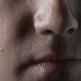
dipole diffusion |

beam diffusion |
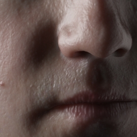
beam diffusion with singlescatter |
Beginning with PRMan 18.0, the "smooth" parameter is useful for reducing noise with ray-traced subsurface(); it used to be only used for point-based but ignored for ray-traced.
Also beginning with PRMan 18.0, there is a new "switchtobrdf" parameter. It enables an optimization based on the observation that if the diffuse mean free path is much shorter than a pixel, then the subsurface scattering will look the same as good old-fashioned Lambertian diffuse reflection. If a distant object has subsurface scattering that looks just the same as diffuse reflection, then we can save a lot of time by just computing diffuse reflection instead. The "switchtobrdf" parameter is a float that specifies a fraction of a pixel size where - if the diffuse mean free path when projected onto the screen is shorter than that size - you permit the subsurface() function to switch to a fast diffuse brdf calculation instead of the full subsurface scattering bssrdf calculation. The default value for "switchtobrdf" is 0.0 for backwards compatibility; reasonable values to get optimal benefit without visible differences are in the 0.25 to 0.5 range. (Implementation detail: the diffuse calculation is done by shooting a single ray back to the shading point and computing diffuse reflection, instead of shooting many rays to sample the subsurface scattering from the entire surface.)
See the standard shader plausibleSubSurface.sl for an example of a shader using ray-traced subsurface scattering.
6.2 Point-based subsurface()
The new subsurface scattering models can also be used with point clouds. As before, the point cloud(s) should represent the direct illumination on the surface of the object. Note that it is still important to generate the point cloud with subsurface scattering in mind: the shader must use area(P, "dicing") to get the correct micropolygon areas and bake3d(..., "interpolate", 1, ...) to bake one point per micropolygon, and the RIB file must set Attribute "dice" "rasterorient" 0 (to turn view-dependent dicing off), Attribute "cull" "hidden" 0, and Attribute "cull" "backfacing" 0 (to avoid culling hidden and backfacing surfaces).
7 ptfilter
The stand-alone program ptfilter can also use the new single-scattering and diffusion scattering models. The scattering parameters are specified as before: a material name or scattering and absorption parameters or albedo and diffusemeanfreepath values - specified on the command line or read from the point cloud file. The type of scattering can be requested in the filter type: -filtertype singlescatter or -filtertype beamdiffusion or -filtertype singlescatter,beamdiffusion for both. The classic dipole type can be specified with -filtertype ssdiffusion (as before) or -filtertype dipolediffusion.
The image below shows a marble teapot with subsurface scattering computed with the following ptfilter command:
ptfilter -filter singlescatter,beamdiffusion -material marble -threads 8 -progress 2 -maxsolidangle 1.0 -smooth 1 direct_rad_t.ptc beamdiffusion.ptc
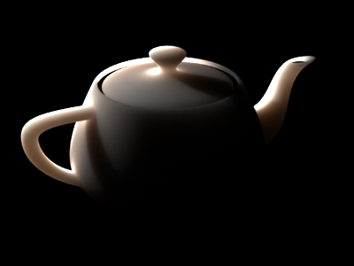
beamdiffusion and singlescatter computed with ptfilter
8 Performance
Due to various optimizations and the use of table lookups, beam diffusion (with single scattering) is typically only around 15 percent slower than dipole diffusion. But in practice, many people have found that they needed to compute two dipole diffusions: one with very short dmfp to simulate single-scattering, and one with longer dmfp to simulate multi-scattering. If comparing two dipole diffusion computations with one beam diffusion with single scattering, the latter is clearly faster.
9 References
More information about the classic dipole approximation of subsurface scattering can be found in the following publications:
| [Jensen01] | (1, 2, 3, 4) Henrik Wann Jensen, Stephen R. Marschner, Marc Levoy, and Pat Hanrahan. A Practical Model for Subsurface Light Transport. Proceedings of SIGGRAPH 2001, pages 511-518. |
| [Jensen02] | Henrik Wann Jensen and Juan Buhler. A Rapid Hierarchical レンダリング Technique for Translucent マテリアル. Proceedings of SIGGRAPH 2002, pages 576-581. |
| [Hery03] | Christophe Hery. Implementing a Skin BSSRDF. In "RenderMan, Theory and Practice", SIGGRAPH 2003 Course Note #9, pages 73-88. |
Multipoles were discussed in this paper (as well as several follow-up papers):
| [Donner05] | Craig Donner and Henrik Wann Jensen. Light Diffusion in Multi-layered Translucent マテリアル. Proceedings of SIGGRAPH 2005, pages 1032-1039. |
The quantized diffusion model was introduced in this paper:
| [dEon11] | (1, 2, 3) Eugene d'Eon and Geoffrey Irving. A Quantized-Diffusion Model for レンダリング Translucent マテリアル. Proceedings of SIGGRAPH 2011, article 56. |
The details of the beam diffusion formulas and methods are described here:
| [Habel13] | Ralf Habel, Per H. Christensen, and Wojciech Jarosz. Photon Beam Diffusion: A Hybrid Monte Carlo Method for Subsurface Scattering<http://graphics.pixar.com/library/PhotonBeamDiffusion/paper.pdf>. Proceedings of EGSR 2013. |
MCML is a Monte Carlo simulation tool used in the biomedical field:
| [Wang95] | Lihong Wang, Steven Jacques, and Liqiong Zheng. MCML -- Monte Carlo Modeling of Light Transport in Multi-layered Tissues. Computer Methods in Programs and Biomedicine 47, 8, pages 313-371. |
10 Appendix A
In general, we would recommend the plausibleSubSurface shader as a clean and consistent example for how to shade surfaces with subsurface scattering.
However, to render the image in section 3 with the various types of subsurface scattering we needed a shader that can compute both diffuse reflection and subsurface scattering (which is normally considered a "dirty hack" - subsurface scattering should replace diffuse reflection to be consistent, not be added to it). Here are the shaders used for that image:
// A circle of light with uniform color
light
circlelight(
  float intensity = 1;
  color lightcolor = 1;
  point center = point(0);
  float radius = 1)
{
  vector dir = vector(0,0,1);
  point Pw = transform("world", Ps);
  float radius2 = radius*radius, deltax, deltay, distxy2, distxy;

  solar(dir, 0) {
      deltax = Pw[0] - center[0];
      deltay = Pw[1] - center[1];
      distxy2 = deltax*deltax + deltay*deltay;
      Cl = filterstep(distxy2,radius2);
      Cl *= intensity * lightcolor;
  }
}

// Subsurface scattering bssrdf, diffuse brdf, specular brdf
// (plausibleSubSubface is a cleaner and more general subsurface shader.)
surface
sssdemo(string type = "";
      color scattering = color(2.19, 2.62, 3.00);
      color absorption = color(0.0021, 0.0041, 0.0071);
      float ior = 1.5;
      float g = 0; // for single-scattering phase function
      float samples = 64;
      float Ks = 0, Kd = 0, Ksss = 1,
      roughness = 0.1; )
{
  normal Nn = normalize(N); // assumes all normals face out of object
  vector Vn = -normalize(I);
  color amb, diff = 0, spec = 0, sss = 0;
  string raylabel;

  rayinfo("label", raylabel);

  if (raylabel != "subsurface") {
    // Compute specular surface reflection (brdf)
    if (Ks > 0) {
      spec = specular(Nn,Vn,roughness);
    }
    // Compute diffuse surface reflection (brdf)
    // (Normally one should not add diffuse and subsurface; pick one)
    if (Kd > 0) {
      diff = diffuse(Nn);
    }
    // Compute ray-traced subsurface scattering bssrdf: singlescatter
    // and/or dipole diffusion or beamdiffusion
    if (Ksss > 0) {
      sss = subsurface("raytraced",
                       P, Nn,
                       "type", type,
                       "scattering", scattering,
                       "absorption", absorption,
                       "ior", ior, "g", g,
                       "samples", samples);
    }
    Ci = Ks*spec + Kd*diff*Cs + Ksss*sss;
  } else {
    // Compute direct illumination (ambient and diffuse; no specular)
    // on the outside of the surface.
    // (Note that there is no mult by Cs here -- if there were, we'd
    // be multiplying by the surface color both going in and out of
    // the surface, leading to too saturated a color.
    // Alternatively, multiply by sqrt(Cs) both going in and out.)
    amb = ambient();
    diff = diffuse(Nn);    // (or -Ns if shadingnormal used)
    Ci = amb + diff;
  }

  // Set Ci and Oi
  Ci *= Os;
  Oi = Os;
}
The RIB file is:
FrameBegin 1

Format 340 340 1
シェーディングInterpolation "smooth"
シェーディングRate 0.25   # to avoid aliasing on circlelight edge on matte material
PixelSamples 6 6
PixelFilter "box" 1 1
Display "square_ssstypes1" "it" "rgba"
Projection "perspective" "fov" 15.4895
Translate 0 0 100

WorldBegin

  Attribute "visibility" "diffuse" 1
  Attribute "trace" "bias" 0.0001

  # Light source
  LightSource "circlelight" 1
    "float intensity" 2.5
    "point center" [0 0 0]
    "float radius" 8

  # Surface strips with various subsurface scattering models

  # --- Top row: single scattering ---

  # Ideal diffuse brdf
  AttributeBegin
    カラー 0.071 0.062 0.050   # attempt at matching MC single-scattering color
    Surface "sssdemo"
      "float Kd" 1.0 "float Ksss" 0.0
    Polygon "P" [ -12 12 0  0 12 0  0 4 0  -12 4 0 ]
  AttributeEnd

  # New diffuse single-scattering model
  AttributeBegin
    Surface "sssdemo"
      "string type" "singlescatter"
      "color scattering" [0.74 0.88 1.01]
      "color absorption" [0.032 0.17 0.48]
      "float ior" 1.3
      "float samples" 600
    Polygon "P" [ 0 12 0  12 12 0  12 4 0  0 4 0 ]
  AttributeEnd

  # --- Middle row: diffusion approximations of multiple scattering ---

  # Classic dipole diffusion model
  AttributeBegin
    Surface "sssdemo"
      "float Ksss" 0.82
      "string type" "dipolediffusion"   # same as "ssdiffusion"
      "color scattering" [0.74 0.88 1.01]
      "color absorption" [0.032 0.17 0.48]
      "float ior" 1.3
      "float samples" 600
    Polygon "P" [ -12 4 0  0 4 0  0 -4 0  -12 -4 0 ]
  AttributeEnd

  # New diffusion model
  AttributeBegin
    Surface "sssdemo"
      "float Ksss" 0.95   # beam diffusion peak is a bit too bright
      "string type" "beamdiffusion"
      "color scattering" [0.74 0.88 1.01]
      "color absorption" [0.032 0.17 0.48]
      "float ior" 1.3
      "float samples" 600
    Polygon "P" [ 0 4 0  12 4 0  12 -4 0  0 -4 0 ]
  AttributeEnd

  # --- Bottom row: single- plus multiscattering ---

  # Dipole diffusion and matte
  AttributeBegin
    カラー 0.65 0.25 0.10   # attempt at matching MC all-scattering color
    Surface "sssdemo"
      "float Kd" 0.1 "float Ksss" 0.82
      "string type" "dipolediffusion"   # same as "ssdiffusion"
      "color scattering" [0.74 0.88 1.01]
      "color absorption" [0.032 0.17 0.48]
      "float ior" 1.3
      "float samples" 600
    Polygon "P" [ -12 -4 0  0 -4 0  0 -12 0  -12 -12 0 ]
  AttributeEnd

  # New diffusion model and diffuse single scattering
  AttributeBegin
    Surface "sssdemo"
      "float Ksss" 0.95   # beam diffusion peak is a bit too bright
      "string type" "beamdiffusion,singlescatter"
      "color scattering" [0.74 0.88 1.01]
      "color absorption" [0.032 0.17 0.48]
      "float ior" 1.3
      "float samples" 600
    Polygon "P" [ 0 -4 0  12 -4 0  12 -12 0  0 -12 0 ]
  AttributeEnd

WorldEnd
FrameEnd